Run SEFRA model

Load packages required for data preparation:

library(dplyr)
library(tidyr)
library(kableExtra)
library(sf)
library(ggplot2)

library(sefra)
library(sefraInputs)

Prelims

Source data from sefraInputs:

sefra_data("inputsBio")

## Loaded data:

## 
## 
## |name      |description |created             |version                | id|
## |:---------|:-----------|:-------------------|:----------------------|--:|
## |inputsBio |reference   |2025-03-27 11:25:55 |20250327T112555Z-ed41c |  2|

sefra_data("cryptic_capture_longline")

## Loaded data:

## 
## 
## |name                     |description |created             |version                | id|
## |:------------------------|:-----------|:-------------------|:----------------------|--:|
## |cryptic_capture_longline |reference   |2025-03-27 11:25:55 |20250327T112555Z-240cc |  1|

Extract biological data for reference case:

# Import demographic data
N_BP       <- inputsBio[["N_BP"]]
S_opt      <- inputsBio[["S_opt"]]
A_curr     <- inputsBio[["A_curr"]]
P_B        <- inputsBio[["P_B"]]
P_nest     <- inputsBio[["p_nest"]]
P_southern <- inputsBio[["p_southern"]]

The `sefraData` object

Data are stored in a S4 object of class sefraData. The sefraData object is a list with pre-defined components. When assigning data to this list, checks are made during the assignment to ensure the data are in the correct format for model input. The sefraData object is initialised using a call to sefraData(<species>, <identifier>). A vector of species must be supplied (see ?species for a list of those available). By defining the species, all subsequent assignments can be checked for consistency with this species list. An identifier argument is also allowed, so that different data configurations can be labelled. In this vignette, we demonstrate how an sefraData object can be populated and input to a model run.

First, initialise the data object using three example species:

sefra_dat <- sefraData(c('DIW', 'DQS', 'TWD'), name = "reference")

## species codes input: including all species-dependent capture codes

## constructed 'sefraData' object

When choosing the species we are assuming that all captures are from one of these species, even if the capture code recorded in the capture data refers to a lower taxonomic resolution. In the example below, captures are also recorded using the generic BLZ code. The model will assume that genus-, family- or generic-level captures are of DIW, DQS or TWD; i.e., when fitting to the data the captures will be predicted from the fishery overlap with these species only. If generic captures could be of other species not recorded at the species level, then these species should be included in the sefraData object. In which case the model will select a zero probability of observation for that species.

Following initialisation of the sefraData object, the species names are available using the accessor function:

species_names(sefra_dat)

## Species

##    code                        common_name                    scientific_name
## 1   DIW                 Gibson's albatross      Diomedea antipodensis gibsoni
## 2   DQS               Antipodean albatross Diomedea antipodensis antipodensis
## 13  TWD New Zealand white-capped albatross          Thalassarche cauta steadi
##           genus      family code_resolution id_species
## 1      Diomedea Diomedeidae         species          1
## 2      Diomedea Diomedeidae         species          2
## 13 Thalassarche Diomedeidae         species         13

which can be useful for labeling plots of model diagnostics. Note that the id_species corresponds to the order recorded in ?species. This numbering is retained throughout, allowing the data inputs and model outputs to be matched consistently to the species.

The relevant capture codes are automatically generated from the list of species, and will include the species-level capture codes, but also lower level taxonomic codes. In the current example:

capture_codes(sefra_dat)

## 10 capture codes:

## (empty captures data frame)

##    code id_code resolution id_resolution
## 1   DIW       1    species             1
## 2   DQS       2    species             1
## 3   TWD      13    species             1
## 4   DGA      26    complex             2
## 5   DST      29    complex             2
## 6   DWC      32    complex             2
## 7   DIZ      34      genus             3
## 8   THZ      35      genus             3
## 9   ALZ      38     family             4
## 10  BLZ      40      class             5

Assign biological data

From the inputsBio data accessed using sefraInputs::sefra_data(), we assign these to the sefraData object. Assignment functions are provided for each data type, and automatically select the required species:

n_breeding_pairs(sefra_dat) <- N_BP       
adult_survival(sefra_dat)   <- S_opt      
p_breeding(sefra_dat)       <- P_B        
age_breeding(sefra_dat)     <- A_curr     
p_nest(sefra_dat)           <- P_nest
p_southern(sefra_dat)       <- P_southern

Biological inputs for the number of breeding pairs, the adult survival, the probability of breeding, and the age at first breeding should be provided as two-parameter probability density functions. These can be one of: uniform, beta, normal, log-normal or logit-normal (see ?distributions). The input data frame must contain the column headers distribution, par1 and par2.

We can view the input data using, for example:

N_BP %>% select(id_species, code, distribution, par1, par2)

##    id_species code distribution       par1      par2
## 1           1  DIW   log-normal    4425.00     0.050
## 2           2  DQS   log-normal    3383.00     0.050
## 3           3  DIX   log-normal   10130.00     0.050
## 4           4  DBN      weibull       9.25  1710.000
## 5           5  DAM   log-normal      60.00     0.100
## 6           6  DIP   log-normal    5814.00     0.070
## 7           7  DIQ   log-normal    4261.00     0.110
## 8           8  DCR   log-normal   26800.00     0.100
## 9           9  TQH   log-normal   33988.00     0.100
## 10         10  DIM   log-normal  670960.00     0.050
## 11         11  TQW   log-normal   14129.00     0.050
## 12         12  DCU   log-normal   15335.00     0.100
## 13         13  TWD   log-normal   85820.00     0.120
## 14         14  DKS   log-normal   35242.00     0.050
## 15         15  DER   log-normal    5294.00     0.010
## 16         16  DIC   log-normal   63055.00     0.050
## 17         17  DSB   log-normal   13493.00     0.050
## 18         18  DNB   log-normal   19354.00     0.050
## 19         19  PHU      weibull      23.20 13660.000
## 20         20  PHE   log-normal   20927.00     0.100
## 21         21  PCI   log-normal  105617.00     0.150
## 22         22  PRK   log-normal    5456.00     0.057
## 23         23  PCW   log-normal    6223.00     0.061
## 24         24  PRO   log-normal 1317300.00     0.100
## 25         25  PCN   log-normal   42000.00     0.096

The assigned model values are:

n_breeding_pairs(sefra_dat)

##     distribution  par1 par2
## DIW   log-normal  4425 0.05
## DQS   log-normal  3383 0.05
## TWD   log-normal 85820 0.12

Similarly:

P_B %>% select(id_species, code, distribution, par1, par2)

##    id_species code distribution  par1    par2
## 1           1  DIW         beta 0.595  170.00
## 2           2  DQS         beta 0.450   91.30
## 3           3  DIX logit-normal 0.494    0.05
## 4           4  DBN         beta 0.349   51.30
## 5           5  DAM logit-normal 0.600    0.05
## 6           6  DIP         beta 0.531   22.20
## 7           7  DIQ         beta 0.531   22.20
## 8           8  DCR         beta 0.596 4100.00
## 9           9  TQH logit-normal 0.596    0.05
## 10         10  DIM         beta 0.844  174.00
## 11         11  TQW logit-normal 0.900    0.05
## 12         12  DCU logit-normal 0.747    0.05
## 13         13  TWD         beta 0.680   63.90
## 14         14  DKS         beta 0.821   29.70
## 15         15  DER logit-normal 0.773    0.05
## 16         16  DIC         beta 0.406   17.50
## 17         17  DSB         beta 0.804   34.90
## 18         18  DNB logit-normal 0.800    0.05
## 19         19  PHU logit-normal 0.730    0.05
## 20         20  PHE         beta 0.730   15.80
## 21         21  PCI logit-normal 0.900    0.05
## 22         22  PRK         beta 0.610  143.00
## 23         23  PCW         beta 0.480   45.40
## 24         24  PRO logit-normal 0.750    0.05
## 25         25  PCN logit-normal 0.797    0.05

p_breeding(sefra_dat)

##     distribution  par1  par2
## DIW         beta 0.595 170.0
## DQS         beta 0.450  91.3
## TWD         beta 0.680  63.9

If you wish to use alternate biological data values, please provide these directly to the project team for inclusion in the sefraInputs package. This will ensure they are available to all participants. Centralisation of the data inputs further allows for consistent cross referencing of different data supplied to different model runs.

Fisheries and structural data

Fisheries input data are stored in the sefraData object in three data frames:

observed captures:
observed overlap
commercial (total) overlap

All the supplied data frames should contain the following headers:

month as a character vector and/or id_month as an integer value between 1 and 12 (see ?months);
year a an integer value;
fishery_group as a character vector and/or id_fishery_group as integer values.

In addition, the captures data frame must include the following field headers:

code as a character vector and/or id_code as integer values (see ?codes for permitted capture codes);
n_captures,
n_captures_alive and,
n_captures_dead as integer values.

The overlap data frames should include:

species as a character vector and/or id_species as integer values (see ?species for permitted capture codes);
species_group as a character vector and/or id_species_group as integer values;
cell and/or id_cell as an integer value between 1 and 1224, this being the number of 5x5 degree cells in the southern hemisphere. For assignment of data to cells, please see the documentation for the sefraInputs package.

All months are referenced using an integer value between 1 and 12. This is true regardless of whether a character vector is supplied. Similarly, all species are referenced using an integer value between 1 and 25, and this id_species value is retained throughout the assessment. The capture code is referenced using an integer value for id_code between 1 and 40, which is similarly retained throughout the assessment and will be consistent across different model runs or data constructs. If you wish to included additional species or capture codes please contact the project team.

There are no fixed reference values for the fishery group or species group, since these are dependent on the analysis and must be provided by the investigator (see the vignette for sefraInputs).

Assignment functions are provided for the species group and fishery group. These represent structural assumptions and must be supplied to the sefraData object before the overlap and capture data frames. This two-step process facilitates checking of the data.

To illustrate, we first create some artificial data, as three separate data frames: captures_o, overlap_o and overlap_t.

Header from observed captures data frame
n_captures	cell	year	code	month	flag	n_captures_dead	id_month	id_fishery_group
0	708	2016	DQS	Jun	F1	0	6	1
0	691	2018	DQS	Jun	F1	0	6	1
1	684	2008	DIW	Mar	F1	1	3	1
0	687	2007	TWD	Jan	F1	0	1	1
0	688	2012	DQS	Dec	F2	0	12	2
0	770	2020	BLZ	Aug	F2	0	8	2

Header from observed overlap data frame
id_species	id_month	id_fishery_group	id_species_group	year	cell	overlap
2	6	1	2	2016	708	0.0004098
2	6	1	2	2018	691	0.0002191
1	3	1	1	2008	684	0.0003939
13	1	1	3	2007	687	0.0005376
2	12	2	2	2012	688	0.0008761
2	8	2	2	2020	770	0.0008146

Header from commercial (total) overlap data frame
id_species	id_month	id_fishery_group	id_species_group	year	cell	overlap
2	6	1	2	2016	708	0.0008923
2	6	1	2	2018	691	0.0007787
1	3	1	1	2008	684	0.0002149
13	1	1	3	2007	687	0.0004784
2	12	2	2	2012	688	0.0007050
2	8	2	2	2020	770	0.0001145

Functions are provided to assign structural assumptions based on the input data frames. For example, we can assign fishery groups using:

fishery_groups(sefra_dat) <- captures_o
fishery_groups(sefra_dat)

## 2 fishery groups

##   fishery_group id_fishery_group
## 1     fishery_1                1
## 2     fishery_2                2

This does not assign any actual data. It only extracts structural information from the data captures_o data frame. Structural assumptions can also be provided as character vectors. In this case, care must be taken to ensure the values match the values in the corresponding input data frames. To specify species groups for example, we could use:

species_groups(sefra_dat) <- c('group_1', 'group_2', 'group_3')

The same results could be achieved by assigning a data frame directly, which is the recommended approach. In this case:

species_groups(sefra_dat) <- overlap_o
species_groups(sefra_dat)

## 3 species groups

##   species_group id_species_group
## 1       group_1                1
## 2       group_2                2
## 3       group_3                3

When examining the species group assignments to each species, we can use:

species_groups(sefra_dat, print_species = TRUE)

## 3 species groups

## (with 3 species)

##   species species_group id_species id_species_group
## 1     DIW       group_1          1                1
## 2     DQS       group_2          2                2
## 3     TWD       group_3         13                3

The data frames themselves can then be assigned. In the first instance, overlap and captures data are provided:

sefra_dat <- sefra_dat %>% data_prep(overlap_o, captures_o)

## Prepared observer captures and overlap data

In this case, two separate data frames are supplied to the data_prep() function. Multiple, data frame can be provided, as long as the referencing is consistent. It is the presence of captures (i.e., n_captures) in at least one of the data frames that identifies the data as observed. Otherwise it is treated as commercial overlap data.

Following assignment of capture data, the captures per code can be viewed using:

capture_codes(sefra_dat)

## 10 capture codes:

## Joining with `by = join_by(id_code)`

##    code id_code resolution id_resolution captures
## 1   DIW       1    species             1       27
## 2   DQS       2    species             1       26
## 3   TWD      13    species             1       23
## 4   DGA      26    complex             2        0
## 5   DST      29    complex             2        0
## 6   DWC      32    complex             2        0
## 7   DIZ      34      genus             3       21
## 8   THZ      35      genus             3       10
## 9   ALZ      38     family             4        0
## 10  BLZ      40      class             5       21

or by taxonomic resolution using:

capture_resolutions(sefra_dat)

## 10 capture code resolutions:

## Joining with `by = join_by(id_fishery_group, id_code)`

##    id_fishery_group id_resolution resolution captures
## 1                 1             1    complex        0
## 2                 1             1    species       12
## 3                 1             2      genus       10
## 4                 1             2    species       13
## 5                 1             3      genus        3
## 6                 1             3    species       11
## 7                 1             4    complex        0
## 8                 1             4     family        0
## 9                 1             5      class       13
## 10                1             5    complex        0
## 11                2             1    complex        0
## 12                2             1    species       15
## 13                2             2      genus       11
## 14                2             2    species       13
## 15                2             3      genus        7
## 16                2             3    species       12
## 17                2             4    complex        0
## 18                2             4     family        0
## 19                2             5      class        8
## 20                2             5    complex        0

In the latter case, captures are disaggregated by fishery group.

To assign the commercial overlap data use:

sefra_dat <- sefra_dat %>% data_prep(overlap_t)

## Prepared commercial (total) overlap data

To check the data have loaded correctly we can view the object:

sefra_dat

## 'sefraData' class object:

## Species

##    code                        common_name                    scientific_name
## 1   DIW                 Gibson's albatross      Diomedea antipodensis gibsoni
## 2   DQS               Antipodean albatross Diomedea antipodensis antipodensis
## 13  TWD New Zealand white-capped albatross          Thalassarche cauta steadi
##           genus      family code_resolution id_species
## 1      Diomedea Diomedeidae         species          1
## 2      Diomedea Diomedeidae         species          2
## 13 Thalassarche Diomedeidae         species         13

## 3 species groups

## (with 3 species)

##   species species_group id_species id_species_group
## 1     DIW       group_1          1                1
## 2     DQS       group_2          2                2
## 3     TWD       group_3         13                3

## 2 fishery groups

##   fishery_group id_fishery_group
## 1     fishery_1                1
## 2     fishery_2                2

## 10 capture codes:

## Joining with `by = join_by(id_code)`

##    code id_code resolution id_resolution captures
## 1   DIW       1    species             1       27
## 2   DQS       2    species             1       26
## 3   TWD      13    species             1       23
## 4   DGA      26    complex             2        0
## 5   DST      29    complex             2        0
## 6   DWC      32    complex             2        0
## 7   DIZ      34      genus             3       21
## 8   THZ      35      genus             3       10
## 9   ALZ      38     family             4        0
## 10  BLZ      40      class             5       21

## Captures data frame:

## # A tibble: 78 × 6
##    captures_k captures_live_k captures_dead_k code_k month_k fishery_group_k
##         <int>           <int>           <int>  <int>   <int>           <int>
##  1          1               1               0      1       1               1
##  2          1               1               0      1       2               1
##  3          2               1               1      1       3               1
##  4          1               1               0      1       5               1
##  5          2               1               1      1       6               1
##  6          1               1               0      1       7               1
##  7          1               1               0      1      10               1
##  8          1               0               1      1      11               1
##  9          2               1               1      1      12               1
## 10          3               2               1      1       1               2
## # ℹ 68 more rows

## Observed overlap data frame:

## # A tibble: 72 × 5
##    overlap_i species_i species_group_i month_i fishery_group_i
##        <dbl>     <int>           <int>   <int>           <int>
##  1   0.00776         1               1       1               1
##  2   0.00139         1               1       2               1
##  3   0.00568         1               1       3               1
##  4   0.00831         1               1       4               1
##  5   0.00541         1               1       5               1
##  6   0.00697         1               1       6               1
##  7   0.00956         1               1       7               1
##  8   0.00770         1               1       8               1
##  9   0.00740         1               1       9               1
## 10   0.00486         1               1      10               1
## # ℹ 62 more rows

## Commercial overlap data frame:

## # A tibble: 962 × 5
##    overlap_j species_j species_group_j month_j fishery_group_j
##        <dbl>     <int>           <int>   <int>           <int>
##  1 0.000384          1               1       1               1
##  2 0.000196          1               1       1               1
##  3 0.000258          1               1       1               1
##  4 0.0000644         1               1       1               1
##  5 0.000763          1               1       1               1
##  6 0.000477          1               1       1               1
##  7 0.000584          1               1       1               1
##  8 0.000653          1               1       1               1
##  9 0.000618          1               1       1               1
## 10 0.000430          1               1       1               1
## # ℹ 952 more rows

Captures and overlap data can also be extracted using, respectively:

captures(sefra_dat)

## # A tibble: 78 × 6
##    captures_k captures_live_k captures_dead_k code_k month_k fishery_group_k
##         <int>           <int>           <int>  <int>   <int>           <int>
##  1          1               1               0      1       1               1
##  2          1               1               0      1       2               1
##  3          2               1               1      1       3               1
##  4          1               1               0      1       5               1
##  5          2               1               1      1       6               1
##  6          1               1               0      1       7               1
##  7          1               1               0      1      10               1
##  8          1               0               1      1      11               1
##  9          2               1               1      1      12               1
## 10          3               2               1      1       1               2
## # ℹ 68 more rows

overlap(sefra_dat)

## $observer
## # A tibble: 72 × 5
##    overlap_i species_i species_group_i month_i fishery_group_i
##        <dbl>     <int>           <int>   <int>           <int>
##  1   0.00776         1               1       1               1
##  2   0.00139         1               1       2               1
##  3   0.00568         1               1       3               1
##  4   0.00831         1               1       4               1
##  5   0.00541         1               1       5               1
##  6   0.00697         1               1       6               1
##  7   0.00956         1               1       7               1
##  8   0.00770         1               1       8               1
##  9   0.00740         1               1       9               1
## 10   0.00486         1               1      10               1
## # ℹ 62 more rows
## 
## $fishery
## # A tibble: 962 × 5
##    overlap_j species_j species_group_j month_j fishery_group_j
##        <dbl>     <int>           <int>   <int>           <int>
##  1 0.000384          1               1       1               1
##  2 0.000196          1               1       1               1
##  3 0.000258          1               1       1               1
##  4 0.0000644         1               1       1               1
##  5 0.000763          1               1       1               1
##  6 0.000477          1               1       1               1
##  7 0.000584          1               1       1               1
##  8 0.000653          1               1       1               1
##  9 0.000618          1               1       1               1
## 10 0.000430          1               1       1               1
## # ℹ 952 more rows

Cryptic capture

Cryptic capture distribution parameters are defined by species group and fishery group, and can be assigned as follows:

cryptic_capture(sefra_dat)  <- cryptic_capture_longline

## 2 fishery groups

## 3 species groups

cryptic_capture(sefra_dat)

##    distribution fishery_group species_group  par value
## 1    log-normal     fishery_1       group_1 par1 1.420
## 2    log-normal     fishery_2       group_1 par1 1.420
## 3    log-normal     fishery_1       group_2 par1 1.420
## 4    log-normal     fishery_2       group_2 par1 1.420
## 5    log-normal     fishery_1       group_3 par1 1.420
## 6    log-normal     fishery_2       group_3 par1 1.420
## 7    log-normal     fishery_1       group_1 par2 0.186
## 8    log-normal     fishery_2       group_1 par2 0.186
## 9    log-normal     fishery_1       group_2 par2 0.186
## 10   log-normal     fishery_2       group_2 par2 0.186
## 11   log-normal     fishery_1       group_3 par2 0.186
## 12   log-normal     fishery_2       group_3 par2 0.186

At present, only a log-normal distribution is allowed. Values stored in the the cryptic_capture_longline object represent the authors best understanding of cryptic capture in longline fisheries, but can be adjusted as required by the user. We have stratified the cryptic captures assumption by species group, because we are currently not aware of any information that would allow a higher resolution.

Example model run

First, source and compile the model code:

sefra_mdl <- sefraModel(sefra_dat)

## SEFRA-seabird model v3.0.1

The sefraModel() function can optionally be supplied with the sefraData-class object as an argument. If commercial overlap is missing from the data, then predicted captures, deaths and risk are not calculated by the model. Only catchabilities and fits to the observed captures will be generated. This will lower the memory requirements for the model and may be useful for initial model-based explorations of the data.

Note that a custom model can also be provided to sefraModel(). In this instance we recommend first calling sefraModel(write_to = <file>) to write the stan code as a text file. This base code can then be modified by the user and re-compiled using sefraModel(read_from = <file>).

The sefraModel-class object will contain the initial values. These can be updated using initial_values() to generate a maximum posterior density estimate. To check initial values:

sefra_mdl <- initial_values(sefra_dat, sefra_mdl)

## initial model fit ✔

This can be useful for quickly exploring the structural assumptions of the model, and whether reasonable fits to the data are obtained. Typically, structural mis-specification of the species and fishery groups, or a deficiency in the data, will lead to stronger prior updates on the biological parameters.

When fitting, the model attempts to reconstruct the number of captures by estimating the catchabilities and observation probabilities according to the structural assumptions implemented by the user. In addition to estimating direct fits to the data, the model also calculates the cumulative sum of the captures, which can be used to examine whether the total number of captures per taxonomic group is being accurately predicted. In particular, we would hope that the total number of captures across all taxonomic groups is accuratly predicted by the model, which can be determined from the models ability to predict the cumulative sum of BLZ captures.

To calculate the cumulative sum of the capture data, captures are summed per fishery group and capture code. Following summation, capture codes represent all captures at that taxonomic resolution or higher. For example, using the current data, the captures per capture code and fishery group are represented within the model as a two-dimensional matrix, with the fishery groups along the first dimension:

## `summarise()` has grouped output by 'id_fishery_group'. You can override using
## the `.groups` argument.
## Joining with `by = join_by(id_fishery_group, code)`

##           DIW DQS TWD DGA DST DWC DIZ THZ ALZ BLZ
## fishery_1  12  13  11   0   0   0  10   3   0  13
## fishery_2  15  13  12   0   0   0  11   7   0   8

The cumulative sum (or “inclusive sum”) of the capture codes used for fitting the model are:

##           DIW DQS TWD DGA DST DWC DIZ THZ ALZ BLZ
## fishery_1  12  13  11  25  11  25  35  14  49  62
## fishery_2  15  13  12  28  12  28  39  19  58  66

For the BLZ capture code, there are 21 captures recorded as BLZ in the empirical data, but a total of 128 BLZ captures when summed across captures recorded as BLZ or a higher taxonomic resolution. We refer to 21 as the empirical captures and 128 as the inclusive captures. Similarly for DIZ we have 21 empirical captures and 74 inclusive captures. This definition of inclusive captures is relevant to the model fit and downstream diagnostics.

Model run

Sample from the posterior using the $sampling() function from cmdstanr:

sefra_mdl <- sampler(sefra_dat, sefra_mdl, chains = 2, parallel_chains = 2, iter_warmup = 1000, iter_sampling = 1000, threads_per_chain = 2)

The different scales on which biological parameters are estimated can make it difficult for the MCMC chain to explore the full parameter space, and the user may therefore wish to adjust the adapt_delta, stepsize or max_treedepth control parameters. We further recommend that uniform priors should only be used for p_breeding and adult_survival (if at all) and not for n_breeding_pairs or age_breeding.

Functions exist to extract and summarise relevant model outputs, to allow the user to create their own diagnostic plots and tables:

sefra_out <- sefraOutputs(sefra_dat, sefra_mdl)

## constructed 'sefraOutputs' object ✔

out_summary <- summary(sefra_out)

PST
species	mean	mq	lq	uq
DIW	306.7724	303.7025	229.7858	403.6591
DQS	285.8586	280.6301	207.6187	390.3796
TWD	6662.0626	6533.0709	4318.3926	9876.8959

Risk ratio
species	mean	mq	lq	uq
DIW	0.0089556	0.0087423	0.0054751	0.0140560
DQS	0.0105234	0.0101956	0.0058968	0.0173810
TWD	0.0004815	0.0004625	0.0002683	0.0008196

Model diagnostics

Trace plots can be used to visualise convergence. For example, we can plot trace diagnostics for the biological parameters using, for example:

trace_plot(sefra_mdl, pars = c("p_breeding"), labels = list(species = paste0("P[", sefra_dat$species, "]")))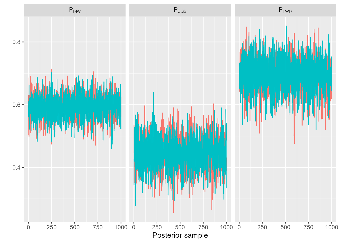

#trace_plot(mdl_fit, pars = c("age_breeding"), labels = list(species = paste0("alpha[", sefra_dat$species, "]")))
#trace_plot(mdl_fit, pars = c("adult_survival"), labels = list(species = paste0("S[", sefra_dat$species, "]")))
#trace_plot(mdl_fit, pars = c("n_breeding_pairs"), labels = list(species = paste0("N[", sefra_dat$species, "]")))

the probabilities of observation:

trace_plot(sefra_mdl, pars = c("p_obs_logit"), labels = list(fishery_group = sefra_dat$fishery_groups, pi = paste("pi[", 1:sefra_dat$n_pi, "]"), resolution = as.character(unique(sefra_dat$resolutions))))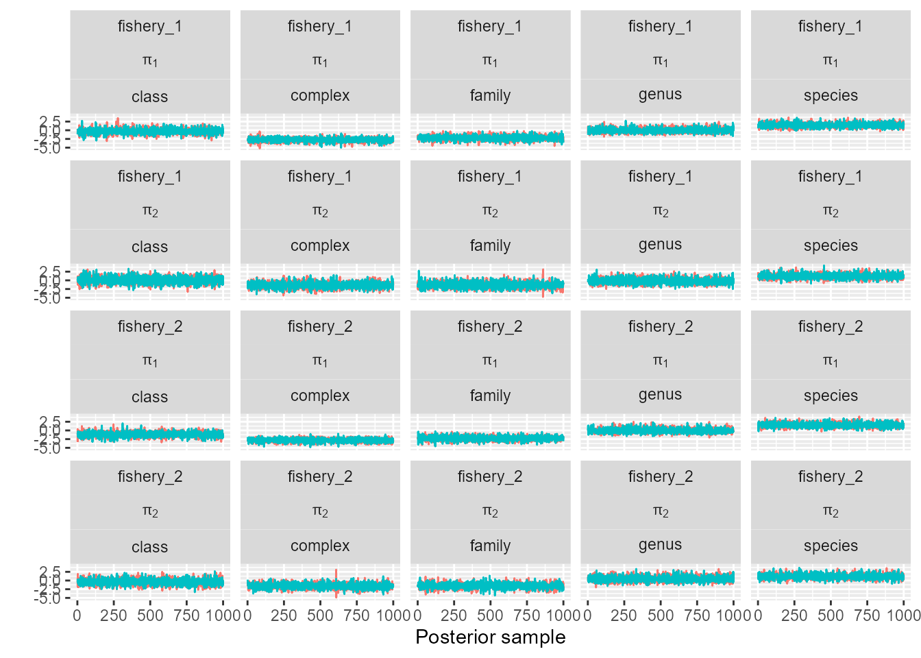

or the catchabilities:

trace_plot(sefra_mdl, pars = "q", labels = list(fishery_group = sefra_dat$fishery_groups, species_group = sefra_dat$species_groups))

To visualise prior updates to the biological input distributions, we use, for example:

plot_prior_update(sefra_mdl, par = "n_breeding_pairs", species_labels = as.character(sefra_dat$species))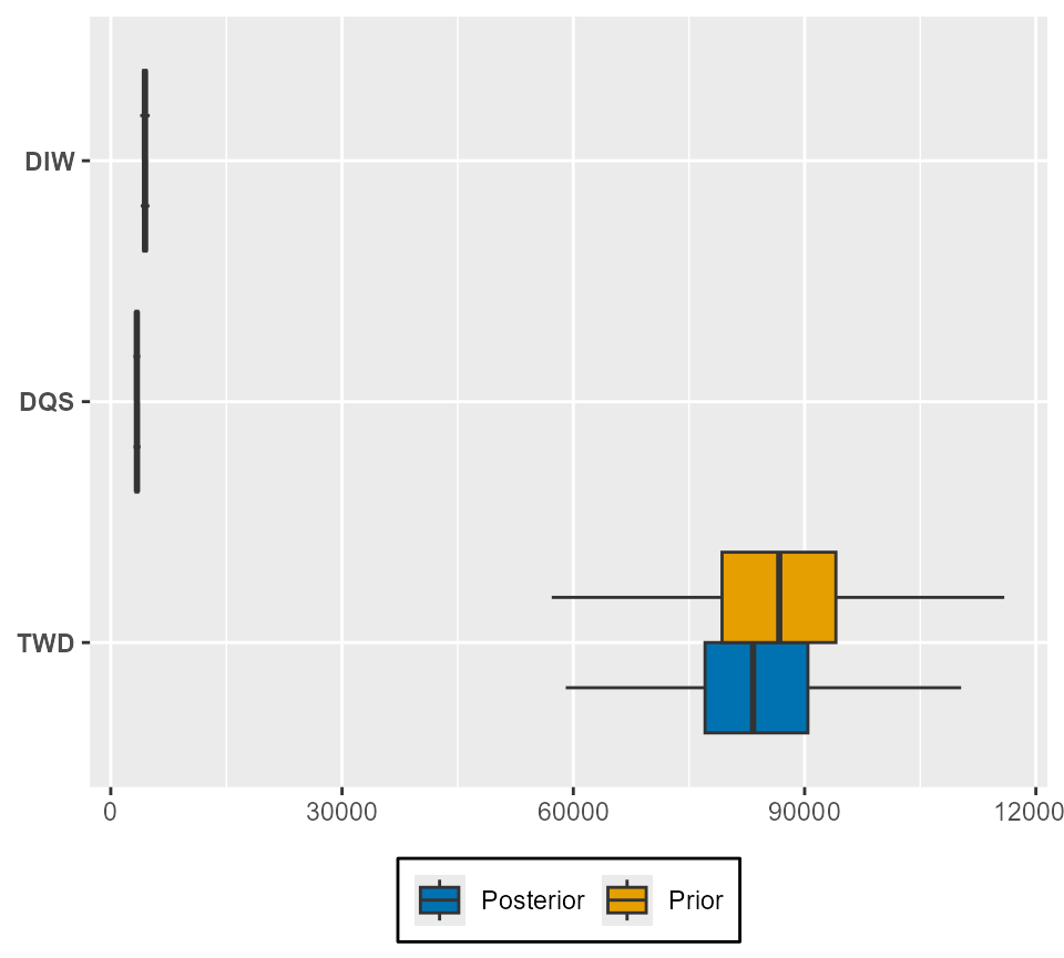

Only one biological parameter can be included per box-plot.

Diagnostic plots also exist for Rhat and Neff. For example:

par_labels <- expression(alpha[1][","][1], alpha[2][","][1], alpha[1][","][2], alpha[2][","][2], alpha[1][","][3], alpha[2][","][3])

plot_rhat(get_traces(sefra_mdl, pars = c("alpha_species_group"), dimnames = list(fishery_group = sefra_dat$fishery_groups, species_group = sefra_dat$species_groups))[[1]], labels = par_labels)

plot_neff(get_traces(sefra_mdl, pars = c("alpha_species_group"), dimnames = list(fishery_group = sefra_dat$fishery_groups, species_group = sefra_dat$species_groups))[[1]], labels = par_labels)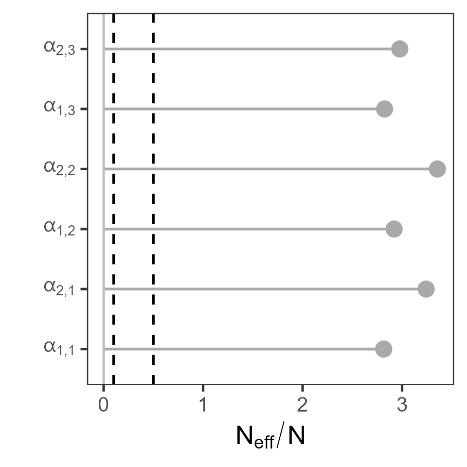

Perhaps the most useful diagnostic is provided from examination of fits to the capture data, and a specific function exists for this purpose:

captures(sefra_dat, sefra_mdl)

## $captures
## # A tibble: 20 × 7
##    fishery_group code  captures hat_mean hat_mq hat_lq hat_uq
##    <chr>         <chr>    <int>    <dbl>  <dbl>  <dbl>  <dbl>
##  1 fishery_1     DIW         12     8.46      8      2   17  
##  2 fishery_1     DQS         13     9.03      9      3   18  
##  3 fishery_1     TWD         11     6.85      6      1   14  
##  4 fishery_1     DGA          0     1.44      1      0    5  
##  5 fishery_1     DST          0     1.97      2      0    6  
##  6 fishery_1     DWC          0     1.45      1      0    5  
##  7 fishery_1     DIZ         10    10.5      10      3   20  
##  8 fishery_1     THZ          3     3.92      4      0   10  
##  9 fishery_1     ALZ          0     4.52      4      0   11  
## 10 fishery_1     BLZ         13    13.8      13      5   25  
## 11 fishery_2     DIW         15    10.3      10      3   20  
## 12 fishery_2     DQS         13     8.93      9      2   18  
## 13 fishery_2     TWD         12     8.19      8      2   16  
## 14 fishery_2     DGA          0     1.46      1      0    5  
## 15 fishery_2     DST          0     2.19      2      0    7  
## 16 fishery_2     DWC          0     1.48      1      0    5  
## 17 fishery_2     DIZ         11    11.4      11      4   21  
## 18 fishery_2     THZ          7     6.51      6      1   14  
## 19 fishery_2     ALZ          0     4.66      4      0   11.0
## 20 fishery_2     BLZ          8    10.7      10      4   20  
## 
## $captures_inclusive
## # A tibble: 20 × 7
##    fishery_group code  captures hat_mean hat_mq hat_lq hat_uq
##    <chr>         <chr>    <int>    <dbl>  <dbl>  <dbl>  <dbl>
##  1 fishery_1     DIW         12     8.48      8      2   17  
##  2 fishery_1     DQS         13     9.01      9      2   18.0
##  3 fishery_1     TWD         11     6.74      6      1   14  
##  4 fishery_1     DGA         25    18.9      18      9   32  
##  5 fishery_1     DST         11     8.79      8      2   18  
##  6 fishery_1     DWC         25    20.2      20     10   33  
##  7 fishery_1     DIZ         35    30.8      30     17   48  
##  8 fishery_1     THZ         14    12.7      12      5   23  
##  9 fishery_1     ALZ         49    48.1      48     30   69  
## 10 fishery_1     BLZ         62    62.1      62     41   87  
## 11 fishery_2     DIW         15    10.3      10      3   20  
## 12 fishery_2     DQS         13     8.89      8      3   18  
## 13 fishery_2     TWD         12     8.19      8      2   17  
## 14 fishery_2     DGA         28    20.8      20     10   35  
## 15 fishery_2     DST         12    10.4      10      4   19.0
## 16 fishery_2     DWC         28    22.1      21     11   36  
## 17 fishery_2     DIZ         39    33.5      33     20   51  
## 18 fishery_2     THZ         19    16.9      16      7   29  
## 19 fishery_2     ALZ         58    54.9      54     37   76  
## 20 fishery_2     BLZ         66    65.8      65     45   89

Further diagnostic are provided in an accompanying vignette.

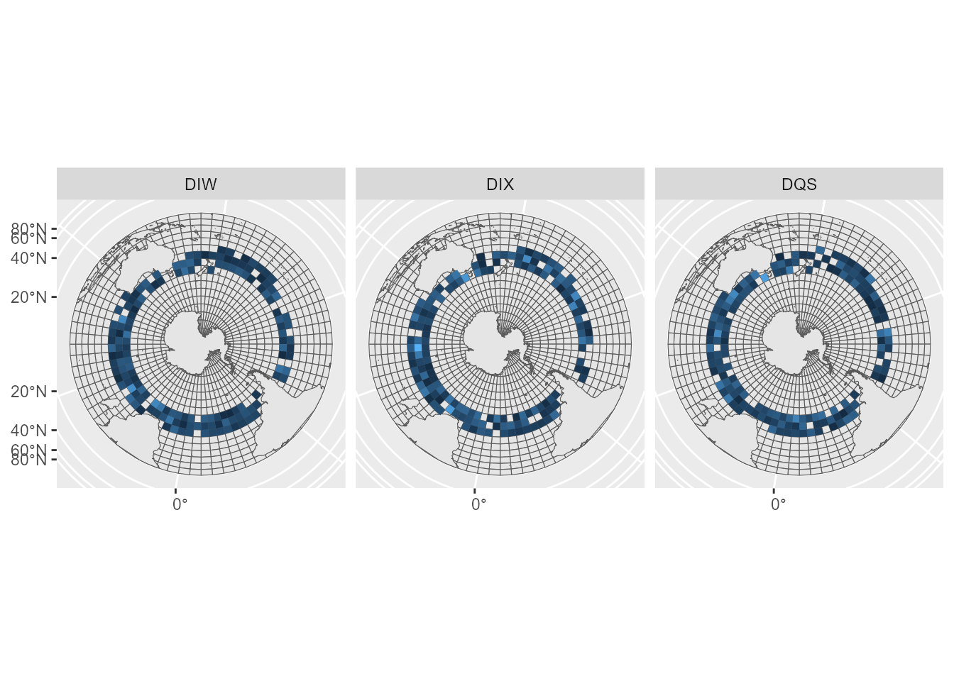
To reconstruct maps, we can use values stored in the sefraOutputs object.

# reconstruct maps

map_deaths <- sefra_out$predicted_deaths %>% group_by(iter, species, cell) %>% summarise(value = sum(value)) %>% group_by(species, cell) %>% summarise(value = median(value))

## `summarise()` has grouped output by 'iter', 'species'. You can override using
## the `.groups` argument.
## `summarise()` has grouped output by 'species'. You can override using the
## `.groups` argument.

map_deaths <- sefraInputs::grid %>% left_join(map_deaths, by = c("id_cell" = "cell")) %>% filter(!is.na(species))

ggplot(map_deaths) + geom_sf(data = sefraInputs::grid)+ geom_sf(data = sefraInputs::southern_map) + geom_sf(aes(fill = value), col = NA) + facet_wrap(~species) + guides(fill = "none")

Charles Edwards and Tom Peatman

31 Dec 2025

Prelims

The `sefraData` object

Assign biological data

Fisheries and structural data

Cryptic capture

Example model run

Model run

Model diagnostics

Run SEFRA model

Charles Edwards and Tom Peatman

31 Dec 2025

Prelims

The sefraData object

Assign biological data

Fisheries and structural data

Cryptic capture

Example model run

Model run

Model diagnostics

The `sefraData` object