Create SEFRA inputs

Tom Peatman and Charles Edwards

06-Apr-2025

Introduction

This vignette provides an example of the preparation of observed captures and effort for incorporation in the 2025 CCSBT collaborative seabird risk assessment, applied to a simple synthetic dataset. The overall approach is identical to that used for the 2024 CCSBT seabird risk assessment, apart from the process of loading in biological data inputs. This has been updated to allow members to prepare their observed captures and effort datasets using different sets of biological inputs, e.g., different seabird density layers. There has also been a minor change to the arguments of get_overlap, which is also described below.

Set up an R session for data preparation

Load packages required for data preparation and visualisation:

library(sefraInputs)
library(ggplot2)
library(sf)
library(kableExtra)
library(dplyr)
library(tidyr)

sf::sf_use_s2(FALSE)
options(dplyr.summarise.inform = FALSE)

Create a local directory in which to save the groomed data necessary for analysis. For the current demonstration, we use the temporary folder generated as part of the active R session:

dir_data <- file.path(tempdir(), "data")

The dir_data directory should not have any groomed data or outputs from previous data preparation attempts, to avoid issues with version control. The following will remove all ‘R’ data (i.e. files with .rda or .RData extensions) and TeX (.tex extensions) files in the dir_data folder and any sub-folders:

make_folder(dir_data, clean = TRUE)

## directory created

Here, we define characters that should not be used in User defined names, e.g. for species groups, fishery groups, time periods, etc.:

latex_special_characters <- paste0(c("\\$", "\\&", "\\_", "\\{"), collapse = "|")
punctuation_characters <- "[[:punct:]]"

Minimum data requirements

Raw observed effort and seabird captures data from pelagic longliners should be stored and accessed using custom scripts developed by the User. We recommend that observed effort and observed seabird captures are sourced separately, and we will assume this to be the case.

The minimum requirements for these data are described here, with required column headers:

• Both the observed effort and captures data must include variables for: flag (ISO 3166-1 alpha-3 country code), year, month, latitude (lat) and longitude (lon). Additional covariates will be required if they are needed to define fishery_group for the purposes of estimating catchabilities. Typically, fishery_group will be defined by the flag, but it is possible to define the fishery group using other covariates, e.g. target species.

• Observed effort should be provided with units of thousand hooks (observer_effort). Observer effort can be summed per flag, year, month, lat, lon and fishery_group to reduce file size.

• Observed captures should be provided with variables for species code (code), status at-vessel (status = alive, dead or NA for unknown), and number of individuals captured (n_captures). Information on age-class of captures should also be provided where available (age_class = adult, immature, juvenile, NA). Although this information is not currently incorporated in the risk assessment model, inclusion of data on the age-class of captures will allow the preparation of high-level summaries of captures by age-class.

• The lat and lon covariates must correspond to the centre of a 5x5 degree spatial grid or finer, to be compatible with the seabird density maps. See the ‘Spatial grid definition’ section for more information on the spatial structure of observer data. The observer data can be provided by the User at any spatial resolution, so long as each record can be attributed to a single cell in (see ?grid). Because the population density maps are at a 5x5 degree resolution, and the data are summed across space to create a measure of overlap, there is no advantage to preparing the data at a finer resolution.

• The temporal resolution of the observer data must be (at a minimum) by year and month, to be compatible with the seabird density maps.

• To ensure that catchabilities are correctly estimated, the catch and effort data must be correctly matched. This means that the capture data must be from strata represented in the observer effort data, and that matching columns contain equivalent information in an equivalent format. As part of the data grooming process, observed captures are linked to the corresponding observed effort, and an identical stratification of the data is therefore necessary. If there are captures outside of the spatial or temporal range of the observer effort data, these captures should be removed until the source of the error is identified. This forms a part of data preparation scripts below.

Check observer data meet minimum requirements

Get totals for initial observed effort and captures. These allow the effects of data filtering to be reported:

N_EFFORT   <- sum(obs_effort$observer_effort)
N_CAPTURES <- sum(obs_captures$n_captures)

Functions check_obs_effort and check_obs_captures should be used to ensure that the observer data meet the minimum requirements:

check_observed_effort(obs_effort)
check_observed_captures(obs_captures)

Additionally, the User may also assign check_observed_effort and check_observed_captures to filter out NAs in the appropriate variables:

obs_effort   <- check_observed_effort(obs_effort)
obs_captures <- check_observed_captures(obs_captures)

The stratification of obs_effort and obs_captures should be identical, and there should not be strata with observed captures but no observed effort.

Get the variables that define the stratification of the observer data (strata_vars), and ensure that they are present in both the observer effort and capture data:

# Variables that define stratification of observed effort data
strata_vars <- colnames(obs_effort)[!colnames(obs_effort) %in% "observer_effort"]
stopifnot(all(strata_vars %in% colnames(obs_effort), strata_vars %in% colnames(obs_captures)))

Check that each record in obs_captures matches at most one record in obs_effort:

obs_effort %>% left_join(., obs_captures, by = strata_vars, relationship = "one-to-many") %>% invisible(.)

This will return an error if a record in obs_captures matches multiple records in obs_effort (due to the relationship argument).

There should not be multiple records in the observer effort data for a particular strata, as this would introduce duplication in captures data when they are joined:

# effort records per strata
effort_records_per_strata <- obs_effort %>%
  group_by_at(., strata_vars) %>%
  summarise(., n = n())

stopifnot(max(effort_records_per_strata$n) == 1)

Filter out captures for strata with no corresponding observed effort data:

obs_captures <- obs_captures %>% semi_join(., obs_effort, by = strata_vars)

Summarise remaining observed effort and captures after initial filtering:

message("Retained effort accounts for ", round(100 * sum(obs_effort$observer_effort)/N_EFFORT, 1), "% of total observed effort provided by User")
message("Retained captures account for ", round(100 * sum(obs_captures$n_captures)/N_CAPTURES, 1), "% of total observed captures provided by User")

Synthetic datasets used in this vignette

In this vignette, we demonstrate how data can be prepared and saved to the directory dir_data on the User’s machine, using the synthetic data provided with this package build. The synthetic data consists of two files:

• Observed effort data in obs_effort.

• Observed seabird captures in obs_captures.

These are loaded into the current R session, for demonstration of the code:

data(obs_effort, obs_captures)

The synthetic observed effort and captures data have the following structure:

Headers for observed effort (synthetic data)

flag	target	year	month	lon	lat	observer_effort
NZL	BET+YFT	2020	1	72.5	-32.5	100
NZL	ALB	2020	4	77.5	-32.5	130
NZL	ALB	2020	7	82.5	-32.5	160
NZL	BET+YFT	2020	10	87.5	-32.5	190
NZL	BET+YFT	2021	1	72.5	-27.5	200
NZL	ALB	2021	4	77.5	-27.5	230

Headers for observed captures (synthetic data)

flag	target	year	month	lon	lat	code	status	age_class	n_captures
NZL	ALB	2020	4	77.5	-32.5	DIW	alive	adult	2
NZL	ALB	2020	4	77.5	-32.5	DIW	alive	immature	1
NZL	ALB	2020	4	77.5	-32.5	DIW	dead	NA	1
NZL	ALB	2020	4	77.5	-32.5	DIW	NA	NA	1
NZL	ALB	2020	4	77.5	-32.5	DIW	alive	adult	1
NZL	ALB	2020	4	77.5	-32.5	DIW	alive	NA	2

The synthetic data are provided at a 5x5 degree spatial resolution, where the longitude and latitude fields provide the mid-point of the 5 degree square grid cell.

Check that synthetic observer data meet minimum requirements

Get totals for initial observed effort and captures:

N_EFFORT   <- sum(obs_effort$observer_effort)
N_CAPTURES <- sum(obs_captures$n_captures)

obs_effort   <- check_observed_effort(obs_effort)
obs_captures <- check_observed_captures(obs_captures)

Get the variables that define the stratification of the observer data (strata_vars), and ensure that they are present in both the observer effort and capture data:

strata_vars <- colnames(obs_effort)[!colnames(obs_effort) %in% "observer_effort"]
stopifnot(all(strata_vars %in% colnames(obs_effort), strata_vars %in% colnames(obs_captures)))

Check that each record in obs_captures matches at most one record in obs_effort:

obs_effort %>% left_join(., obs_captures, by = strata_vars, relationship = "one-to-many") %>% invisible(.)

Check for multiple records in the observer effort data for a particular strata, which would introduce duplication in captures data when they are joined:

# effort records per strata
effort_records_per_strata <- obs_effort %>%
  group_by_at(., strata_vars) %>%
  summarise(., n = n())

stopifnot(max(effort_records_per_strata$n) == 1)

Filter out captures for strata with no corresponding observed effort data:

obs_captures <- obs_captures %>% semi_join(., obs_effort, by = strata_vars)

Summarise remaining observed effort and captures after initial filtering:

## Observed effort after check_observed_effort accounts for 100% of total observed effort provided by User

## Observed captures after check_observed_effort and check_observed_captures accounts for 100% of total observed captures provided by User

Access biological input data for the risk assessment model

As described above, this section has been updated for the 2025 CCSBT risk assessment, to allow preparation of data inputs with different sets of biological inputs.

Biological input data for the risk assessment model, including demographic parameters and seabird density maps, are available through the sefraInputs package. The biological inputs can be accessed using the sefra_data function.

Calling the sefra_data function with no arguments returns a summary of available biological inputs:

## Available SEFRA data:

##                       name                        description
## 1                inputsBio                     2024_CCSBT_SRA
## 2                inputsBio                          reference
## 3 cryptic_capture_longline                          reference
## 4             density_maps                     2024_CCSBT_SRA
## 5             density_maps 2024_CCSBT_SRA_combined_range_maps
## 6             density_maps                          reference
## 7             density_maps      reference_combined_range_maps
##               created                version id
## 1 2025-03-27 12:25:55 20250327T112555Z-1dd6f  1
## 2 2025-03-27 12:25:55 20250327T112555Z-ed41c  2
## 3 2025-03-27 12:25:55 20250327T112555Z-240cc  1
## 4 2025-03-27 12:26:01 20250327T112601Z-e6ac4  1
## 5 2025-03-27 12:26:02 20250327T112602Z-80743  2
## 6 2025-03-27 12:26:03 20250327T112603Z-92e7d  3
## 7 2025-03-27 12:26:04 20250327T112604Z-a6ad2  4

Other data objects that are required, or helpful, when preparing data inputs can be accessed through a call to data(). To check what data are available in the current package build, use:

data(package = "sefraInputs")

Demographic parameters

To load the current biological inputs into the global environment (i.e., the inputsBio object) , we select the object where description = "reference":

sefra_data("inputsBio", description = "reference")

## Loaded data:

## 
## 
## |name      |description |created             |version                | id|
## |:---------|:-----------|:-------------------|:----------------------|--:|
## |inputsBio |reference   |2025-03-27 12:25:55 |20250327T112555Z-ed41c |  2|

The biological inputs for the 2024 CCSBT risk assessment are also available (i.e., description = "2024_CCSBT_SRA"). Biological inputs will updated and added the sefraInputs package as the project progresses.

inputsBio is a list object, with each element providing the inputs for one biological or demographic variable. Each set of biological inputs contains the following data frames: sp_codes, sp_groups, breeding_season, p_nest, breeding_phenology, p_southern, N_BP, P_B, S_curr, S_opt, A_curr, A_opt. This approach is intended to facilitate data preparation with different biological inputs, e.g., for sensitivity analyses.

Here, we prepare the synthetic observer dataset using the current best estimates of the biological inputs:

inputs_bio_option <- inputsBio

Create a separate object for each element of inputs_bio_option:

invisible(sapply(names(inputs_bio_option), function(i) {
  assign(i, value = inputs_bio_option[[i]], envir = .GlobalEnv)
  message("Created ", i)
}))

## Created sp_codes

## Created sp_groups

## Created breeding_season

## Created p_nest

## Created breeding_phenology

## Created p_southern

## Created N_BP

## Created P_B

## Created S_curr

## Created S_opt

## Created A_curr

## Created A_opt

To retrieve the species list:

assign("species", value = inputs_bio_option[["sp_codes"]][,"code"], envir = .GlobalEnv)

Seabird density maps

To load the current seabird density maps into the global environment (i.e., the density_maps object) , we select the object where description = "reference":

sefra_data("density_maps", description = "reference")

## Loaded data:

## 
## 
## |name         |description |created             |version                | id|
## |:------------|:-----------|:-------------------|:----------------------|--:|
## |density_maps |reference   |2025-03-27 12:26:03 |20250327T112603Z-92e7d |  3|

Density maps will updated and added the sefraInputs package as the project progresses, e.g., updated density maps for selected species with additional tracking data, and density maps incorporating range maps from Birdlife International.

Here, we prepare the synthetic observer dataset using the current best estimates of the biological inputs:

density_maps_option <- density_maps

Create a separate object for each element of density_maps:

invisible(sapply(names(density_maps_option), function(i) {
  assign(paste0("densities_", i), value = density_maps_option[[i]], envir = .GlobalEnv)
  message("Created ", paste0("densities_", i))
}))

## Created densities_dam

## Created densities_dbn

## Created densities_dcr

## Created densities_dcu

## Created densities_der

## Created densities_dic

## Created densities_dim

## Created densities_dip

## Created densities_diq

## Created densities_diw

## Created densities_dix

## Created densities_dks

## Created densities_dnb

## Created densities_dqs

## Created densities_dsb

## Created densities_pci

## Created densities_pcn

## Created densities_pcw

## Created densities_phe

## Created densities_phu

## Created densities_prk

## Created densities_pro

## Created densities_tqh

## Created densities_tqw

## Created densities_twd

Spatial grid definition

The seabird density maps all have the same 5 degree spatial structure. This 5 degree grid (called grid) is included in the sefraInputs package, to facilitate the preparation of observed effort data with a spatial structure and coordinate reference system that is consistent with the seabird density maps (see ?grid). This consistency in spatial structures and coordinate reference systems is required to estimate the spatial overlap between fishing effort and seabird populations.

The grid is accessible using:

data("grid", package = "sefraInputs")

The grid is a sf object, with each 5 x 5 degree cell represented as a polygon. The grid has an associated coordinate reference system (see st_crs(grid). During the data preparation, the User’s observer data must be converted to a sf object, with the same coordinate reference system as grid. This is done for the example dataset in Section ‘Format obs_data for calculation of density overlap’.

Seabird species, and species groupings of catchabilities

Species in the risk assessment model

The sp_codes data frame provides numeric species identifiers (id_species), species codes (code - using FAO ASFIS three-alpha codes where available), and common names (common_name), for the seabird species included in the risk assessment model:

sp_codes %>% head(.) %>% kable(.)

id_species	code	common_name
1	DIW	Gibson’s albatross
2	DQS	Antipodean albatross
3	DIX	Wandering albatross
4	DBN	Tristan albatross
5	DAM	Amsterdam albatross
6	DIP	Southern royal albatross

Species groupings for estimation of catchabilities

Catchability parameters define catch rates per unit of observed density overlap. Catchability parameters can be shared across species, e.g. on the basis of similarities in behaviour when attending fishing vessels.

The sp_groups data frame is used to define the species groupings used to estimate catchabilities, i.e., the species_group and id_species_group variables.

The sp_groups object in inputsBio[['reference']] provides the species groupings used in the 2024 seabird risk assessment:

sp_groups %>% filter(., !is.na(id_species_group)) %>%
  select(., id_species_group, species_group) %>% distinct(.) %>%
  arrange(., id_species_group) %>%
  kable(.)

id_species_group	species_group
1	Wandering albatross
2	Royal albatross
3	Small albatross
4	Sooty albatross
5	Medium petrel

However, the species groupings can be updated by the User for application to their observer data (see the following sub-section).

The sp_groups data frame also includes records for seabird captures that were not recorded to a species level. This allows all observed seabird captures to inform the risk assessment model, even if the captures were not identified to a species-level. The variable taxonomic_resolution defines whether the code reflects identifications to a species level, species complex (complex), genus or family level.

The data field fao_code is a logical variable indicating whether the code is a FAO ASFIS code (TRUE) or not (FALSE). id_code provides a unique (integer) identifier for each record.

Codes are also provided for captures that are identified to a finer taxonomic resolution than genus, but a coarser resolution than species. We refer to these as been having identified to a ‘species complex’ level. The following records in sp_groups give the codes that should be used for captures identified to a ‘species complex’ level:

sp_groups %>% filter(., taxonomic_resolution %in% "complex") %>% kable(.)

common_name	scientific_name	genus	family	species_group	catchability_group	capture_group	id_code	id_genus	id_family	code	taxonomic_resolution	fao_code	id_species	id_species_group
Gibson’s and Antipodean albatross	Diomedea antipodensis gibsoni and D. a. antipodensis	Diomedea	Diomedeidae	NA	NA	Great albatross	26	1	1	DGA	complex	FALSE	NA	NA
Royal albatrosses	Diomedea epomophora and D. sanfordi	Diomedea	Diomedeidae	NA	NA	Great albatross	27	1	1	DRA	complex	FALSE	NA	NA
Yellow-nosed albatrosses	Thalassarche chlororhynchos and T. carteri	Thalassarche	Diomedeidae	NA	NA	Mollymawk	28	2	1	DYN	complex	FALSE	NA	NA
Shy-type albatross	Thalassarche cauta and T. c. steadi	Thalassarche	Diomedeidae	NA	NA	Mollymawk	29	2	1	DST	complex	FALSE	NA	NA
Black-browed albatrosses	Thalassarche melanophris and T. impavida	Thalassarche	Diomedeidae	NA	NA	Mollymawk	30	2	1	DBB	complex	FALSE	NA	NA
Buller’s albatross	Thalassarche bulleri bulleri and T. bulleri platei	Thalassarche	Diomedeidae	NA	NA	Mollymawk	31	2	1	DIB	complex	TRUE	NA	NA
Wandering albatross complex	Diomedea exulans, D. dabbenena, D. amsterdamensis, D. antipodensis gibsoni and D. a. antipodensis	Diomedea	Diomedeidae	NA	NA	Great albatross	32	1	1	DWC	complex	FALSE	NA	NA
Petrel complex	Procellaria parkinsoni, P. westlandica and P. aequinoctialis	Procellaria	Procellariidae	NA	NA	Medium petrel	33	4	2	PRZ	complex	FALSE	NA	NA

The following records in sp_groups give the codes that should be used for captures identified to a genus level:

sp_groups %>% filter(., taxonomic_resolution %in% "genus") %>% kable(.)

common_name	scientific_name	genus	family	species_group	catchability_group	capture_group	id_code	id_genus	id_family	code	taxonomic_resolution	fao_code	id_species	id_species_group
Diomedea spp	Diomedea spp	Diomedea	Diomedeidae	NA	NA	Great albatross	34	1	1	DIZ	genus	FALSE	NA	NA
Thalassarche spp	Thalassarche spp	Thalassarche	Diomedeidae	NA	NA	Mollymawk	35	2	1	THZ	genus	FALSE	NA	NA
Phoebetria spp	Phoebetria spp	Phoebetria	Diomedeidae	NA	NA	Sooty albatross	36	3	1	PHZ	genus	FALSE	NA	NA
Procellaria spp	Procellaria spp	Procellaria	Procellariidae	NA	NA	Medium petrel	37	4	2	PTZ	genus	TRUE	NA	NA

The following records in sp_groups give the codes that should be used for captures identified to a family level:

sp_groups %>% filter(., taxonomic_resolution %in% "family") %>% kable(.)

common_name	scientific_name	genus	family	species_group	catchability_group	capture_group	id_code	id_genus	id_family	code	taxonomic_resolution	fao_code	id_species	id_species_group
Diomedeidae	Diomedeidae	NA	Diomedeidae	NA	NA	Unassigned	38	NA	1	ALZ	family	TRUE	NA	NA
Procellariidae	Procellariidae	NA	Procellariidae	NA	NA	Unassigned	39	NA	2	PRX	family	TRUE	NA	NA

There is also a record in sp_groups with the code that should be used for captures that were not identified to a family level:

sp_groups %>% filter(., taxonomic_resolution %in% "bird") %>% kable(.)

common_name	scientific_name	genus	family	species_group	catchability_group	capture_group	id_code	id_genus	id_family	code	taxonomic_resolution	fao_code	id_species	id_species_group

Users must map their species codings for seabird captures to the corresponding values in sp_codes and sp_groups, so that captures are assigned to the correct species group for estimation of catchabilities.

Additional records in sp_groups may be required to facilitate this mapping, for example, if there are captures with codes that reflect identifications to a finer taxonomic resolution than genus, but with a coarser resolution than species. Users should request additional records by creating an Issue for the sefraInputs Github repository.

It is essential that Users request additional records to be added to the sp_groups object in the R package if necessary, rather than working off a modified local version of sp_groups. This will ensure that all members have consistent codes (code) and identifiers (id_code) in their captures datasets.

Updating species groupings for estimation of catchabilities

Species groups may need to be adjusted for application to the User’s observer dataset.

If this is required, the function assign_species_groups should be used to update the sp_groups object, based on a lookup table provided by the User called species_group_definitions. The updated species groups in sp_groups will then propagate through to the observed captures and observed overlap.

The User should not manually adjust species groups directly in the data objects, i.e., do not directly adjust species_group or id_species_group in obs_data, obs_overlap, overlap_o, captures_o, etc.

For example, to define species groups using genus, i.e., grouping all great albatrosses (Diomedea species) together, the User should run the following:

# Initial species groupings
sp_groups_init <- sp_groups

# Updated species group definitions for separate groups per genus
genus_list <- unique(sp_groups$genus)
genus_list <- genus_list[!is.na(genus_list)]
species_group_definitions <- data.frame(id_species_group = 1:length(genus_list), genus = genus_list, species_group = genus_list)

stopifnot(all(!grepl(latex_special_characters, species_group_definitions$species_group)))
stopifnot(all(!grepl(punctuation_characters, species_group_definitions$species_group)))

# Assign updated species groups
sp_groups <- assign_species_groups(sp_groups, species_group_definitions, by = "genus")

Species group names (species_group) can have spaces, but should not have punctuation characters, or special characters in LaTeX, e.g. underscores (_), ampersands (&), dollar signs ($) etc.

To prepare the synthetic data, we use the species groups from the 2024 CCSBT seabird risk assessment. Members should also use these species groups when preparing their data for inclusion in the combined dataset (i.e., the dataset that includes data from all participating members), as consistent species groups must be used by all members.

First, ensure that the sp_groups has not been updated:

if(!isTRUE(all.equal(sp_groups, inputs_bio_option[["sp_groups"]]))) {
  message("Resetting species groups to inputs_bio_option[['sp_groups']]")
  sp_groups <- inputs_bio_option[["sp_groups"]]
}

The species groups are:

kable(sp_groups, caption = "Species groups used to prepare the synthetic dataset.")

Species groups used to prepare the synthetic dataset.

common_name	scientific_name	genus	family	species_group	catchability_group	capture_group	id_code	id_genus	id_family	code	taxonomic_resolution	fao_code	id_species	id_species_group
Gibson’s albatross	Diomedea antipodensis gibsoni	Diomedea	Diomedeidae	Wandering albatross	Wandering albatross	Great albatross	1	1	1	DIW	species	TRUE	1	1
Antipodean albatross	Diomedea antipodensis antipodensis	Diomedea	Diomedeidae	Wandering albatross	Wandering albatross	Great albatross	2	1	1	DQS	species	TRUE	2	1
Wandering albatross	Diomedea exulans	Diomedea	Diomedeidae	Wandering albatross	Wandering albatross	Great albatross	3	1	1	DIX	species	TRUE	3	1
Tristan albatross	Diomedea dabbenena	Diomedea	Diomedeidae	Wandering albatross	Wandering albatross	Great albatross	4	1	1	DBN	species	TRUE	4	1
Amsterdam albatross	Diomedea amsterdamensis	Diomedea	Diomedeidae	Wandering albatross	Wandering albatross	Great albatross	5	1	1	DAM	species	TRUE	5	1
Southern royal albatross	Diomedea epomophora	Diomedea	Diomedeidae	Royal albatross	Royal albatross	Great albatross	6	1	1	DIP	species	TRUE	6	2
Northern royal albatross	Diomedea sanfordi	Diomedea	Diomedeidae	Royal albatross	Royal albatross	Great albatross	7	1	1	DIQ	species	TRUE	7	2
Atlantic yellow-nosed albatross	Thalassarche chlororhynchos	Thalassarche	Diomedeidae	Small albatross	Mollymawk	Mollymawk	8	2	1	DCR	species	TRUE	8	3
Indian yellow-nosed albatross	Thalassarche carteri	Thalassarche	Diomedeidae	Small albatross	Mollymawk	Mollymawk	9	2	1	TQH	species	TRUE	9	3
Black-browed albatross	Thalassarche melanophris	Thalassarche	Diomedeidae	Small albatross	Mollymawk	Mollymawk	10	2	1	DIM	species	TRUE	10	3
Campbell black-browed albatross	Thalassarche impavida	Thalassarche	Diomedeidae	Small albatross	Mollymawk	Mollymawk	11	2	1	TQW	species	TRUE	11	3
Shy albatross	Thalassarche cauta	Thalassarche	Diomedeidae	Small albatross	Mollymawk	Mollymawk	12	2	1	DCU	species	TRUE	12	3
New Zealand white-capped albatross	Thalassarche cauta steadi	Thalassarche	Diomedeidae	Small albatross	Mollymawk	Mollymawk	13	2	1	TWD	species	TRUE	13	3
Salvin’s albatross	Thalassarche salvini	Thalassarche	Diomedeidae	Small albatross	Mollymawk	Mollymawk	14	2	1	DKS	species	TRUE	14	3
Chatham Island albatross	Thalassarche eremita	Thalassarche	Diomedeidae	Small albatross	Mollymawk	Mollymawk	15	2	1	DER	species	TRUE	15	3
Grey-headed albatross	Thalassarche chrysostoma	Thalassarche	Diomedeidae	Small albatross	Mollymawk	Mollymawk	16	2	1	DIC	species	TRUE	16	3
Southern Buller’s albatross	Thalassarche bulleri bulleri	Thalassarche	Diomedeidae	Small albatross	Mollymawk	Mollymawk	17	2	1	DSB	species	FALSE	17	3
Northern Buller’s albatross	Thalassarche bulleri platei	Thalassarche	Diomedeidae	Small albatross	Mollymawk	Mollymawk	18	2	1	DNB	species	FALSE	18	3
Sooty albatross	Phoebetria fusca	Phoebetria	Diomedeidae	Sooty albatross	Sooty albatross	Sooty albatross	19	3	1	PHU	species	TRUE	19	4
Light-mantled sooty albatross	Phoebetria palpebrata	Phoebetria	Diomedeidae	Sooty albatross	Sooty albatross	Sooty albatross	20	3	1	PHE	species	TRUE	20	4
Grey petrel	Procellaria cinerea	Procellaria	Procellariidae	Medium petrel	Medium petrel	Medium petrel	21	4	2	PCI	species	TRUE	21	5
Black petrel	Procellaria parkinsoni	Procellaria	Procellariidae	Medium petrel	Medium petrel	Medium petrel	22	4	2	PRK	species	TRUE	22	5
Westland petrel	Procellaria westlandica	Procellaria	Procellariidae	Medium petrel	Medium petrel	Medium petrel	23	4	2	PCW	species	TRUE	23	5
White-chinned petrel	Procellaria aequinoctialis	Procellaria	Procellariidae	Medium petrel	Medium petrel	Medium petrel	24	4	2	PRO	species	TRUE	24	5
Spectacled petrel	Procellaria conspicillata	Procellaria	Procellariidae	Medium petrel	Medium petrel	Medium petrel	25	4	2	PCN	species	TRUE	25	5
Gibson’s and Antipodean albatross	Diomedea antipodensis gibsoni and D. a. antipodensis	Diomedea	Diomedeidae	NA	NA	Great albatross	26	1	1	DGA	complex	FALSE	NA	NA
Royal albatrosses	Diomedea epomophora and D. sanfordi	Diomedea	Diomedeidae	NA	NA	Great albatross	27	1	1	DRA	complex	FALSE	NA	NA
Yellow-nosed albatrosses	Thalassarche chlororhynchos and T. carteri	Thalassarche	Diomedeidae	NA	NA	Mollymawk	28	2	1	DYN	complex	FALSE	NA	NA
Shy-type albatross	Thalassarche cauta and T. c. steadi	Thalassarche	Diomedeidae	NA	NA	Mollymawk	29	2	1	DST	complex	FALSE	NA	NA
Black-browed albatrosses	Thalassarche melanophris and T. impavida	Thalassarche	Diomedeidae	NA	NA	Mollymawk	30	2	1	DBB	complex	FALSE	NA	NA
Buller’s albatross	Thalassarche bulleri bulleri and T. bulleri platei	Thalassarche	Diomedeidae	NA	NA	Mollymawk	31	2	1	DIB	complex	TRUE	NA	NA
Wandering albatross complex	Diomedea exulans, D. dabbenena, D. amsterdamensis, D. antipodensis gibsoni and D. a. antipodensis	Diomedea	Diomedeidae	NA	NA	Great albatross	32	1	1	DWC	complex	FALSE	NA	NA
Petrel complex	Procellaria parkinsoni, P. westlandica and P. aequinoctialis	Procellaria	Procellariidae	NA	NA	Medium petrel	33	4	2	PRZ	complex	FALSE	NA	NA
Diomedea spp	Diomedea spp	Diomedea	Diomedeidae	NA	NA	Great albatross	34	1	1	DIZ	genus	FALSE	NA	NA
Thalassarche spp	Thalassarche spp	Thalassarche	Diomedeidae	NA	NA	Mollymawk	35	2	1	THZ	genus	FALSE	NA	NA
Phoebetria spp	Phoebetria spp	Phoebetria	Diomedeidae	NA	NA	Sooty albatross	36	3	1	PHZ	genus	FALSE	NA	NA
Procellaria spp	Procellaria spp	Procellaria	Procellariidae	NA	NA	Medium petrel	37	4	2	PTZ	genus	TRUE	NA	NA
Diomedeidae	Diomedeidae	NA	Diomedeidae	NA	NA	Unassigned	38	NA	1	ALZ	family	TRUE	NA	NA
Procellariidae	Procellariidae	NA	Procellariidae	NA	NA	Unassigned	39	NA	2	PRX	family	TRUE	NA	NA
Bird	Aves	NA	NA	NA	NA	Unassigned	40	NA	NA	BLZ	class	FALSE	NA	NA

Save sp_groups and (if necessary) species_groups_definitions for use in the risk assessment model:

save(sp_groups, file = file.path(dir_data, "sp_groups.rda"))
if(exists("species_group_definitions")) {
  save(species_group_definitions, file = file.path(dir_data, "species_group_definitions.rda"))
}

Prepare observed effort and captures data

Specify the time-period for observations used to estimate catchabilities

There is a compromise when specifying the time-period from which observer data are used to estimate catchabilities. Seabird captures are relatively rare, and so longer time-series of observer data may be preferred in order to inform the model. However, earlier observer data may be less reliable, e.g., if observer training on seabird identification and monitoring for seabird captures was less robust in earlier years. Furthermore, population sizes of the birds being caught will have changed over time.

fishing_years_fit defines the years from which observer data are used to estimate catchabilities. This is saved as part of the data preparation process. In our example, we use all available observer data:

fishing_years_fit <- 2020:2021
save(fishing_years_fit, file = file.path(dir_data, "fishing_years_fit.rda"))

The observer data are then filtered to keep data from the appropriate time period:

obs_effort   <- obs_effort %>% filter(., year %in% fishing_years_fit)
obs_captures <- obs_captures %>% filter(., year %in% fishing_years_fit)

Combine observed effort with capture data

Get total observed effort and captures, which will be used to check that total captures have been preserved:

N_EFFORT   <- sum(obs_effort$observer_effort)
N_CAPTURES <- sum(obs_captures$n_captures)

Add the (numeric) code ID (id_code) to the capture data:

obs_captures <- sp_groups %>%
  dplyr::select(., code, id_code) %>%
  left_join(obs_captures, ., by = "code")

Check for observed captures of species codes not included in the risk assessment model:

## Observed captures of species codes not included in the risk assessment model account for 100% of total observed seabird captures

Restructure the captures data to have one record per strata:

obs_captures <- obs_captures %>%
  group_by_at(strata_vars) %>%
  summarise(code = list(code),
            id_code = list(id_code),
            captures_status = list(status),
            age_class = list(age_class),
            n_captures = list(n_captures)) %>%
  data.frame(.)

Combine observed effort and captures, and check that total observed effort and captures have been preserved:

obs_data <- obs_effort %>% left_join(., obs_captures, by = strata_vars)
stopifnot(isTRUE(all.equal(sum(obs_data$observer_effort), N_EFFORT)))
stopifnot(isTRUE(all.equal(sum(unlist(obs_data$n_captures)), N_CAPTURES)))

Add a unique identifier to each record in obs_data called record_id:

obs_data <- obs_data %>% mutate(., record_id = row_number())
obs_data <- obs_data %>% select(., record_id, everything())

The combined observer dataset has the following structure:

obs_data %>% kable(.)

record_id	flag	target	year	month	lon	lat	observer_effort	code	id_code	captures_status	age_class	n_captures
1	NZL	BET+YFT	2020	1	72.5	-32.5	100	NULL	NULL	NULL	NULL	NULL
2	NZL	ALB	2020	4	77.5	-32.5	130	DIW, DIW, DIW, DIW, DIW, DIW, DIZ, BLZ	1, 1, 1, 1, 1, 1, 34, 40	alive, alive, dead , NA , alive, alive, alive, dead	adult , immature, NA , NA , adult , NA , adult , NA	2, 1, 1, 1, 1, 2, 1, 1
3	NZL	ALB	2020	7	82.5	-32.5	160	DCU, DCU, TWD, TWD, TWD, THZ, THZ	12, 12, 13, 13, 13, 35, 35	alive, alive, dead , dead , NA , alive, alive	adult , immature, adult , immature, NA , juvenile, NA	5, 1, 2, 1, 1, 1, 2
4	NZL	BET+YFT	2020	10	87.5	-32.5	190	NULL	NULL	NULL	NULL	NULL
5	NZL	BET+YFT	2021	1	72.5	-27.5	200	PCN, PCN, PCN, PCN, PTZ	25, 25, 25, 25, 37	alive, dead , dead , NA , alive	NA , immature, juvenile, NA , adult	1, 11, 1, 1, 2
6	NZL	ALB	2021	4	77.5	-27.5	230	NULL	NULL	NULL	NULL	NULL
7	NZL	ALB	2021	7	82.5	-27.5	260	NULL	NULL	NULL	NULL	NULL
8	NZL	BET+YFT	2021	10	87.5	-27.5	290	PRO, PRO, PRO, PRO, PCN, PCN, PRX	24, 24, 24, 24, 25, 25, 39	alive, alive, dead , dead , dead , dead , alive	adult , juvenile, adult , NA , adult , immature, adult	2, 1, 9, 1, 9, 2, 2

Assign fishery group IDs

It is necessary to assign ‘fishery groups’ to the observed effort and capture data. Catchabilities are estimated with a fishery group specific parameter, such that different fishery groups are more, or less, likely to capture seabirds, all else being equal. However, all observed effort could be represented by a single fishery group.

The function assign_fishery_groups assigns fishery groups, defined as any combination of variables in the argument lk_definitions. The variables defining fishery groups must be present in both the observer dataset and the dataset of total effort used to estimate total captures.

In this example, we define fishing groups based on target species.

First, create a look-up table called lk_fishery_groups that provides a name for each fishery group (the fishery_group variable):

lk_fishery_groups <- data.frame(id_fishery_group = c(1L, 2L), fishery_group = c("Albacore", "Tropical Tuna"))

stopifnot(all(!duplicated(lk_fishery_groups$id_fishery_group)))
stopifnot(is.integer(lk_fishery_groups$id_fishery_group))
stopifnot(all(!grepl(latex_special_characters, lk_fishery_groups$fishery_group)))
stopifnot(all(!grepl(punctuation_characters, lk_fishery_groups$fishery_group)))

id_fishery_group must be an integer. fishery_group names can have spaces, but should not have punctuation characters, or special characters in LaTeX, e.g. underscores (_), ampersands (&), dollar signs ($) etc.

Then create a data frame called fishery_group_definitions that defines fishery groups, in this case based on target species:

fishery_group_definitions <- data.frame(id_fishery_group = c(1L, 2L), target = c("ALB", "BET+YFT"))
stopifnot(all(fishery_group_definitions$id_fishery_group %in% lk_fishery_groups$id_fishery_group))

The look-up table of fishery group names in this example (lk_fishery_groups) is:

id_fishery_group	fishery_group
1	Albacore
2	Tropical Tuna

and the data frame defining the fishery groups (fishery_group_definitions) is:

id_fishery_group	target
1	ALB
2	BET+YFT

Assign fishery groups to obs_data using assign_fishery_groups:

obs_data <- assign_fishery_groups(obs_data, lk_definitions = fishery_group_definitions, lk_names = lk_fishery_groups)

## Joining with `by = join_by(target)`

As mentioned above, the User can choose to include all surface longline effort in a single fishery group. E.g., for observed effort of Japanese vessels, a single fishery group could be applied with:

lk_fishery_groups <- data.frame(id_fishery_group = 1L, fishery_group = "All")
fishery_group_definitions <- data.frame(id_fishery_group = 1L, flag = "JPN")

obs_data <- assign_fishery_groups(obs_data, lk_definitions = fishery_group_definitions, lk_names = lk_fishery_groups)

Check for observer data with no assigned fishery group:

## Observed effort with an assigned fishery group accounts for 100% of total observed effort
## (and 100% of total observed seabird captures)

Then save fishery_group_definitions and lk_fishery_groups so that fishery groups can be assigned to the total effort data (for the User’s longline fleet):

save(lk_fishery_groups, file = file.path(dir_data, "lk_fishery_groups.rda"))
save(fishery_group_definitions, file = file.path(dir_data, "fishery_group_definitions.rda"))

Assign time periods for catchabilities

Catchabilities can be estimated with time-varying catchabilities, e.g., to reflect changes in seabird bycatch mitigation measures through time. Similarly to fishery groups, the full time series of observer could be considered as a single time period. The function assign_time_periods assigns the periods of time in which catchabilities are shared.

Here, for example purposes, we define separate time periods for 2020 and 2021.

Create a look-up table called lk_time_periods that provides a name for each time period (the period variable):

lk_time_periods <- data.frame(id_period = c(1L, 2L), period = c("early", "late"))

stopifnot(all(!duplicated(lk_time_periods$id_period)))
stopifnot(is.integer(lk_time_periods$id_period))
stopifnot(all(!grepl(latex_special_characters, lk_time_periods$period)))
stopifnot(all(!grepl(punctuation_characters, lk_time_periods$period)))

id_period must be an integer. period names can have spaces, but should not have punctuation characters, or special characters in LaTeX, e.g. underscores (_), ampersands (&), dollar signs ($) etc.

Then, create a data frame called time_period_definitions that defines separate time periods for each year:

time_period_definitions <- data.frame(id_period = c(1L, 2L), year = c(2020L, 2021L))
stopifnot(all(time_period_definitions$id_period %in% lk_time_periods$id_period))

The look-up table of time period names in this example (lk_time_periods) is:

id_period	period
1	early
2	late

and the data frame defining the time periods (time_period_definitions) is:

id_period	year
1	2020
2	2021

Now assign time periods to obs_data using assign_time_period:

obs_data <- assign_time_periods(obs_data, lk_definitions = time_period_definitions, lk_names = lk_time_periods)

## Joining with `by = join_by(year)`

Check for observer data with no assigned time period:

## Observed effort with an assigned time period accounts for 100% of total observed effort
## (and 100% of total observed seabird captures)

Then save time_period_definitions and lk_time_periods so that time periods can be assigned to the total effort dataset (for the User’s longline fleet):

save(lk_time_periods, file = file.path(dir_data, "lk_time_periods.rda"))
save(time_period_definitions, file = file.path(dir_data, "time_period_definitions.rda"))

Remove records missing required information

Remove records missing required information to get observed density overlap with seabird distributions:

obs_data  <- obs_data %>%
  filter(!is.na(month)) %>%
  filter(!(is.na(lat) | is.na(lon)))

## Observed effort with required location and month information accounts for 100% of total observed effort
## (and 100% of total observed seabird captures)

Format obs_data for calculation of density overlap

First, convert month to give the abbreviated month name, keeping month as an integer in a new field called month_id:

obs_data$id_month <- obs_data$month
obs_data$month <- month.abb[obs_data$month]
stopifnot(all(!is.na(obs_data$month)))

The month variable is used to get the seabird density map for the correct month for each record in obs_data.

The synthetic observer data are provided at a 5 degree resolution (matching the spatial resolution of the seabird density maps), with the provided latitude / longitude positions giving the mid-point of the 5 degree cell.

As described above, it is necessary for obs_data to be a sf object, with the correct coordinate reference system, to allow the calculation of overlap between fishing effort and seabird distributions. The spatial information should be included in a variable named geometry.

Reformat obs_data to be a sf object, with the geometry variable representing the location of fishing effort (provided as lat/lons):

obs_data <- obs_data %>%
  rowwise(.) %>%
  mutate(., geometry = list(st_point(c(lon, lat)))) %>%
  ungroup(.) %>%
  st_as_sf(., crs = "EPSG:4326")

The coordinate reference system of obs_data must be transformed to that of grid to ensure a consistent coordinate reference system with the seabird density maps:

obs_data <- obs_data %>% st_transform(crs = st_crs(grid))

It is important to note that, when preparing your own data, the location of fishing effort does not necessarily need to be represented as a point. For example, polygons could be used for aggregated effort data. The most appropriate approach for the User will depend on their data structure, e.g., midpoints of cells or polygons are appropriate for data aggregated to a 1x1 or 5x5 resolution, whereas set locations can be used for set-level observer data.

Add unique cell identifiers from grid to obs_data, to allow for model diagnostics with a spatial dimension:

obs_data <- get_id_cell(obs_data, fun = min)

Points that fall on a boundary between multiple 5 degree cells (i.e. a boundary or intersection between polygons in grid) are assigned the lowest id_cell from matching cells with fun = min in get_id_cell calls. Note that get_overlap uses the mean density across the appropriate cells, for points on a boundary or intersection between multiple 5 degree cells.

The observer data have the following structure:

## sf [8 × 18] (S3: sf/tbl_df/tbl/data.frame)
##  $ record_id       : int [1:8] 1 2 3 4 5 6 7 8
##  $ flag            : chr [1:8] "NZL" "NZL" "NZL" "NZL" ...
##  $ target          : chr [1:8] "BET+YFT" "ALB" "ALB" "BET+YFT" ...
##  $ year            : int [1:8] 2020 2020 2020 2020 2021 2021 2021 2021
##  $ month           : chr [1:8] "Jan" "Apr" "Jul" "Oct" ...
##  $ lon             : num [1:8] 72.5 77.5 82.5 87.5 72.5 77.5 82.5 87.5
##  $ lat             : num [1:8] -32.5 -32.5 -32.5 -32.5 -27.5 -27.5 -27.5 -27.5
##  $ observer_effort : int [1:8] 100 130 160 190 200 230 260 290
##  $ code            :List of 8
##   ..$ : NULL
##   ..$ : chr [1:8] "DIW" "DIW" "DIW" "DIW" ...
##   ..$ : chr [1:7] "DCU" "DCU" "TWD" "TWD" ...
##   ..$ : NULL
##   ..$ : chr [1:5] "PCN" "PCN" "PCN" "PCN" ...
##   ..$ : NULL
##   ..$ : NULL
##   ..$ : chr [1:7] "PRO" "PRO" "PRO" "PRO" ...
##  $ id_code         :List of 8
##   ..$ : NULL
##   ..$ : int [1:8] 1 1 1 1 1 1 34 40
##   ..$ : int [1:7] 12 12 13 13 13 35 35
##   ..$ : NULL
##   ..$ : int [1:5] 25 25 25 25 37
##   ..$ : NULL
##   ..$ : NULL
##   ..$ : int [1:7] 24 24 24 24 25 25 39
##  $ captures_status :List of 8
##   ..$ : NULL
##   ..$ : chr [1:8] "alive" "alive" "dead" NA ...
##   ..$ : chr [1:7] "alive" "alive" "dead" "dead" ...
##   ..$ : NULL
##   ..$ : chr [1:5] "alive" "dead" "dead" NA ...
##   ..$ : NULL
##   ..$ : NULL
##   ..$ : chr [1:7] "alive" "alive" "dead" "dead" ...
##  $ age_class       :List of 8
##   ..$ : NULL
##   ..$ : chr [1:8] "adult" "immature" NA NA ...
##   ..$ : chr [1:7] "adult" "immature" "adult" "immature" ...
##   ..$ : NULL
##   ..$ : chr [1:5] NA "immature" "juvenile" NA ...
##   ..$ : NULL
##   ..$ : NULL
##   ..$ : chr [1:7] "adult" "juvenile" "adult" NA ...
##  $ n_captures      :List of 8
##   ..$ : NULL
##   ..$ : int [1:8] 2 1 1 1 1 2 1 1
##   ..$ : int [1:7] 5 1 2 1 1 1 2
##   ..$ : NULL
##   ..$ : int [1:5] 1 11 1 1 2
##   ..$ : NULL
##   ..$ : NULL
##   ..$ : int [1:7] 2 1 9 1 9 2 2
##  $ id_fishery_group: int [1:8] 2 1 1 2 2 1 1 2
##  $ id_period       : int [1:8] 1 1 1 1 2 2 2 2
##  $ id_month        : int [1:8] 1 4 7 10 1 4 7 10
##  $ geometry        :sfc_POINT of length 8; first list element:  'XY' num [1:2] -6087560 -801442
##  $ id_cell         : int [1:8] 771 772 773 774 843 844 845 846
##  - attr(*, "sf_column")= chr "geometry"
##  - attr(*, "agr")= Factor w/ 3 levels "constant","aggregate",..: NA NA NA NA NA NA NA NA NA NA ...
##   ..- attr(*, "names")= chr [1:17] "record_id" "flag" "target" "year" ...

Generate data inputs for the risk assessment model

Calculate density overlap of observed fishing effort with seabird distributions

Calculate density overlap by species:

obs_overlap <- obs_data %>% select(., record_id, flag, year, id_period, id_month, month, id_fishery_group, id_cell, observer_effort)
for (spp in species) {
  obs_overlap <- obs_overlap %>% get_overlap(., get(paste0("densities_", tolower(spp))), name = spp, effort_name = "observer_effort", group_name = "month")
}

Please note that get_overlap has been updated to take the seabird density map as the y argument, rather than taking the relevant density map from the global environment based on the species code. For more information see ?get_overlap.

Now finished with spatial information in obs_overlap, so remove spatial information:

obs_overlap <- obs_overlap %>% st_drop_geometry(.)
stopifnot(nrow(obs_data) == nrow(obs_overlap))

Aggregate observed density overlap

Create object overlap_o with aggregated observed overlap for model fitting:

# Record for checking
OVERLAP_O <- sum(obs_overlap[, grepl("^overlap_", colnames(obs_overlap))], na.rm = TRUE)

# Generate data frame with aggregated observed overlap by species
overlap_o <- obs_overlap %>% aggregate_overlap(., flag, id_fishery_group, year, id_period, id_month, month, id_cell)

# Add species groups and taxonomic information
overlap_o <- sp_groups %>%
  dplyr::select(., code, id_code, id_species_group, id_species, id_genus, id_family) %>%
  left_join(overlap_o, ., by = "code")

# And reformat variables
overlap_o <- overlap_o %>%
  mutate(id_month = as.integer(id_month),
         id_period = as.integer(id_period),
         id_fishery_group = as.integer(id_fishery_group),
         id_cell = as.integer(id_cell),
         id_code = as.integer(id_code),
         id_species_group = as.integer(id_species_group),
         id_species = as.integer(id_species),
         id_genus = as.integer(id_genus),
         id_family = as.integer(id_family))

# Reorder variables
overlap_o <- overlap_o %>%
  dplyr::select(., flag, id_fishery_group, year, id_period, id_month, month, id_cell,
                code, id_code, id_species_group, id_species, id_genus, id_family, overlap)

# check no NA values
stopifnot(all(!is.na(overlap_o$overlap)))

# check overlap
stopifnot(isTRUE(all.equal(OVERLAP_O, sum(overlap_o$overlap))))

The structure of overlap_o is:

overlap_o %>% str(.)

## tibble [200 × 14] (S3: tbl_df/tbl/data.frame)
##  $ flag            : chr [1:200] "NZL" "NZL" "NZL" "NZL" ...
##  $ id_fishery_group: int [1:200] 1 1 1 1 2 2 2 2 1 1 ...
##  $ year            : int [1:200] 2020 2020 2021 2021 2020 2020 2021 2021 2020 2020 ...
##  $ id_period       : int [1:200] 1 1 2 2 1 1 2 2 1 1 ...
##  $ id_month        : int [1:200] 4 7 4 7 1 10 1 10 4 7 ...
##  $ month           : chr [1:200] "Apr" "Jul" "Apr" "Jul" ...
##  $ id_cell         : int [1:200] 772 773 844 845 771 774 843 846 772 773 ...
##  $ code            : chr [1:200] "DAM" "DAM" "DAM" "DAM" ...
##  $ id_code         : int [1:200] 5 5 5 5 5 5 5 5 4 4 ...
##  $ id_species_group: int [1:200] 1 1 1 1 1 1 1 1 1 1 ...
##  $ id_species      : int [1:200] 5 5 5 5 5 5 5 5 4 4 ...
##  $ id_genus        : int [1:200] 1 1 1 1 1 1 1 1 1 1 ...
##  $ id_family       : int [1:200] 1 1 1 1 1 1 1 1 1 1 ...
##  $ overlap         : num [1:200] 1.88e-05 1.70e-05 1.53e-05 1.41e-05 1.47e-05 ...

overlap_o has a finer stratification than the resolution of the risk assessment model. This allows for more detailed diagnostics of the model fits to observed captures, both temporally and spatially.

Aggregate observed captures to resolution of the risk assessment model

Get captures by ‘species code’, including individuals not identified to a species-level:

# Create a named vector of all codes (used in aggregate_captures call)
named_sp_codes <- sp_groups[, "code"]
names(named_sp_codes) <- named_sp_codes

captures_all <- obs_data %>%
  as.data.frame() %>%
  aggregate_captures(strata = c("flag", "id_fishery_group", "year", "id_period", "id_month", "month", "id_cell"), named_sp_codes) %>%
  rename(., code = group)

Get captures by status (alive / dead):

captures_alive <- obs_data %>% as.data.frame(.) %>%
  filter_captures(., field = "captures_status", condition = "alive") %>%
  aggregate_captures(., strata = c("flag", "id_fishery_group", "year", "id_period", "id_month", "id_cell"), named_sp_codes) %>%
  rename(., code = group)

captures_dead <- obs_data %>% as.data.frame(.) %>%
  filter_captures(., field = "captures_status", condition = "dead")  %>%
  aggregate_captures(., strata = c("flag", "id_fishery_group", "year", "id_period", "id_month", "id_cell"), named_sp_codes) %>%
  rename(., code = group)

captures_status <- full_join(
  captures_alive, captures_dead,
  by = c("flag", "id_fishery_group", "year", "id_period", "id_month", "id_cell", "code"),
  suffix = c("_alive", "_dead"))

## Captures without usable status information (i.e. not 'alive' or 'dead') = 3

Combine observed captures data to include total individuals, and individuals by status:

captures_o <- sp_groups %>%
  dplyr::select(., id_code, id_species_group, id_species, id_genus, id_family, code, taxonomic_resolution) %>%
  left_join(., captures_all, by = "code", relationship = "one-to-many") %>%
  left_join(., captures_status, by = c("flag", "id_fishery_group", "year", "id_period", "id_month", "id_cell", "code"), relationship = "one-to-one")

captures_o <- captures_o %>% select(., flag, id_fishery_group, year, id_period, id_month, month, id_cell,
                                    code, id_code, id_species_group, everything())

For taxonomic ID fields in captures_o, replace NAs with -1’s:

id_vars <- c("id_species", "id_species_group", "id_genus", "id_family")
captures_o[, id_vars] <- lapply(captures_o[, id_vars], function(x) {
  x[is.na(x)] <- -1L
  x
})

The structure of captures_o is:

captures_o %>% str(.)

## 'data.frame':    320 obs. of  17 variables:
##  $ flag                : chr  "NZL" "NZL" "NZL" "NZL" ...
##  $ id_fishery_group    : int  1 1 1 1 2 2 2 2 1 1 ...
##  $ year                : int  2020 2020 2021 2021 2020 2020 2021 2021 2020 2020 ...
##  $ id_period           : int  1 1 2 2 1 1 2 2 1 1 ...
##  $ id_month            : int  4 7 4 7 1 10 1 10 4 7 ...
##  $ month               : chr  "Apr" "Jul" "Apr" "Jul" ...
##  $ id_cell             : int  772 773 844 845 771 774 843 846 772 773 ...
##  $ code                : chr  "DIW" "DIW" "DIW" "DIW" ...
##  $ id_code             : int  1 1 1 1 1 1 1 1 2 2 ...
##  $ id_species_group    : num  1 1 1 1 1 1 1 1 1 1 ...
##  $ id_species          : int  1 1 1 1 1 1 1 1 2 2 ...
##  $ id_genus            : num  1 1 1 1 1 1 1 1 1 1 ...
##  $ id_family           : int  1 1 1 1 1 1 1 1 1 1 ...
##  $ taxonomic_resolution: chr  "species" "species" "species" "species" ...
##  $ n_captures          : int  8 0 0 0 0 0 0 0 0 0 ...
##  $ n_captures_alive    : int  6 0 0 0 0 0 0 0 0 0 ...
##  $ n_captures_dead     : int  1 0 0 0 0 0 0 0 0 0 ...

Similarly to overlap_o, captures_o has a finer stratification than the resolution of the risk assessment model. This allows for more detailed diagnostics of the model fits to observed captures, both temporally and spatially.

Generate tables and figures summarising prepared data

Here, LaTeX tables and figures are generated which summarise the prepared observer dataset. This facilitates generation of standardised tables and figures for all collaborating CCSBT members that provide a broad overview of the analysed datasets. Saving tables in LaTeX format will facilitate composition of the final report. Tables are also saved in binary format for ease of manipulation should alternative presentations be required.

tables_path <- file.path(dir_data, "tables")
make_folder(tables_path)

## directory created

figures_path <- file.path(dir_data, "figures")
make_folder(figures_path)

## directory created

Make a character string with flags, to use when creating table captions etc.:

flag_str <- paste(unique(overlap_o$flag), collapse = ", ")
flag_str_label <- paste(unique(overlap_o$flag), collapse = "-")

Summary tables of observed effort

# Observed effort by year
tab <- obs_data %>%
  st_drop_geometry(.) %>% 
  group_by(., flag, year) %>%
  summarise(., observer_effort = sum(observer_effort)) %>% ungroup(.)

# Drop flag from object used to create kable object
observed_effort <- tab
tab <- tab %>% select(., - flag)

# Format numeric variables
tab <- tab %>% numeric_table_format(., names = "observer_effort", digits = 1)

# Set column names for kable object
kbl_colnames <- stringr::str_to_sentence(colnames(tab))
kbl_colnames <- gsub("_", " ", kbl_colnames)

# caption
kbl_cap <- paste0("Sum of observed fishing effort ('000 hooks) per year for ", flag_str, ".")

tab <- kable(tab, format = 'latex',
       col.names = kbl_colnames,
       row.names = FALSE,
       caption = kbl_cap,
       label = paste0("observed_effort_by_year_", flag_str_label),
       align = c("l", "r"),
       linesep = "", booktabs = TRUE, escape = FALSE) %>% kable_styling(font_size = 10, latex_options = "hold_position") %>%
  sub("\\\\toprule", "", .) %>%
  sub("\\\\bottomrule", "", .)

save_kable(tab, file = file.path(tables_path, "observed_effort_by_year.tex"))
save(observed_effort, file = file.path(tables_path, "observed_effort_by_year.rda"))

flag	year	observer_effort
NZL	2020	580
NZL	2021	980

# Observed effort by year and fishery group
if(nrow(lk_fishery_groups) > 1) {
    
  tab <- obs_data %>%
    st_drop_geometry(.) %>%
    group_by(., flag, year, id_fishery_group) %>%
    summarise(., observer_effort = sum(observer_effort)) %>% ungroup(.)
  tab <- tab %>% left_join(., lk_fishery_groups, by = "id_fishery_group")
  tab <- tab %>% pivot_wider(., id_cols = c(flag, year), names_from = fishery_group, values_from = observer_effort, values_fill = 0)

  # Add a totals column
  tab$total <- rowSums(tab[, !colnames(tab) %in% c("flag", "year")])

  # Drop flag from object used to create kable object
  observed_effort_by_fgroup <- tab  
  tab <- tab %>% select(., - flag)

  # Format numeric variables
  tab <- tab %>% numeric_table_format(., names = c(lk_fishery_groups$fishery_group, "total"), digits = 1)

  # Set column names for kable object
  kbl_colnames <- stringr::str_to_sentence(colnames(tab))

  # caption
  kbl_cap <- paste0("Sum of observed effort ('000 hooks) by fishery group for ", flag_str, ".")

  tab <- kable(tab, format = 'latex',
       col.names = kbl_colnames,
       row.names = FALSE,
       caption = kbl_cap,
       label = paste0("observed_effort_by_fgroup", flag_str_label),
       align = c("l", rep("r", times = ncol(tab) - 1)),
       linesep = "", booktabs = TRUE, escape = FALSE) %>% kable_styling(font_size = 10, latex_options = "hold_position") %>%
  sub("\\\\toprule", "", .) %>%
  sub("\\\\bottomrule", "", .)
  
  save_kable(tab, file = file.path(tables_path, "observed_effort_by_fgroup.tex"))
  save(observed_effort_by_fgroup, file = file.path(tables_path, "observed_effort_by_fgroup.rda"))
}

flag	year	Albacore	Tropical Tuna	total
NZL	2020	290	290	580
NZL	2021	490	490	980

Summary tables of observed captures by code

# Captures by species code (and capture status)
tab <- captures_o %>% group_by(., flag, code) %>% summarise(., across(matches("captures"), sum)) %>% ungroup(.)
tab <- sp_groups %>% select(., code, common_name, taxonomic_resolution) %>%
  left_join(., tab, by = "code") %>%
  select(., flag, code, common_name, taxonomic_resolution, n_captures, n_captures_alive, n_captures_dead)

# Drop flag from object used to create kable object
observed_captures_by_code <- tab
tab <- tab %>% select(., - flag)

# Format numeric variables
tab <- tab %>% numeric_table_format(., names = c("n_captures", "n_captures_alive", "n_captures_dead"), digits = 0)

## New names:
## New names:
## • `` -> `...1`
## • `` -> `...2`
## • `` -> `...3`

# Set column names for kable object
kbl_colnames <- colnames(tab)
kbl_colnames <- gsub("n_captures$", "Total", kbl_colnames)
kbl_colnames <- gsub("n_captures_", "", kbl_colnames)
kbl_colnames <- stringr::str_to_sentence(kbl_colnames)
kbl_colnames <- gsub("_", " ", kbl_colnames)

kbl_cap <- paste0("Sum of observed captures by code for ", flag_str, ".")

tab <- kable(tab, format = 'latex',
       col.names = kbl_colnames,
       row.names = FALSE,
       caption = kbl_cap,
       label = paste0("observed_captures_by_code", flag_str_label),
       align = c("l", "l", "l", "r", "r", "r"),
       linesep = "", booktabs = TRUE, escape = FALSE) %>% kable_styling(font_size = 10, latex_options = "hold_position") %>%
  sub("\\\\toprule", "", .) %>%
  sub("\\\\bottomrule", "", .)
save_kable(tab, file = file.path(tables_path, "observed_captures_by_code.tex"))
save(observed_captures_by_code, file = file.path(tables_path, "observed_captures_by_code.rda"))

flag	code	common_name	taxonomic_resolution	n_captures	n_captures_alive	n_captures_dead
NZL	DIW	Gibson’s albatross	species	8	6	1
NZL	DQS	Antipodean albatross	species	0	0	0
NZL	DIX	Wandering albatross	species	0	0	0
NZL	DBN	Tristan albatross	species	0	0	0
NZL	DAM	Amsterdam albatross	species	0	0	0
NZL	DIP	Southern royal albatross	species	0	0	0
NZL	DIQ	Northern royal albatross	species	0	0	0
NZL	DCR	Atlantic yellow-nosed albatross	species	0	0	0
NZL	TQH	Indian yellow-nosed albatross	species	0	0	0
NZL	DIM	Black-browed albatross	species	0	0	0
NZL	TQW	Campbell black-browed albatross	species	0	0	0
NZL	DCU	Shy albatross	species	6	6	0
NZL	TWD	New Zealand white-capped albatross	species	4	0	3
NZL	DKS	Salvin’s albatross	species	0	0	0
NZL	DER	Chatham Island albatross	species	0	0	0
NZL	DIC	Grey-headed albatross	species	0	0	0
NZL	DSB	Southern Buller’s albatross	species	0	0	0
NZL	DNB	Northern Buller’s albatross	species	0	0	0
NZL	PHU	Sooty albatross	species	0	0	0
NZL	PHE	Light-mantled sooty albatross	species	0	0	0
NZL	PCI	Grey petrel	species	0	0	0
NZL	PRK	Black petrel	species	0	0	0
NZL	PCW	Westland petrel	species	0	0	0
NZL	PRO	White-chinned petrel	species	13	3	10
NZL	PCN	Spectacled petrel	species	25	1	23
NZL	DGA	Gibson’s and Antipodean albatross	complex	0	0	0
NZL	DRA	Royal albatrosses	complex	0	0	0
NZL	DYN	Yellow-nosed albatrosses	complex	0	0	0
NZL	DST	Shy-type albatross	complex	0	0	0
NZL	DBB	Black-browed albatrosses	complex	0	0	0
NZL	DIB	Buller’s albatross	complex	0	0	0
NZL	DWC	Wandering albatross complex	complex	0	0	0
NZL	PRZ	Petrel complex	complex	0	0	0
NZL	DIZ	Diomedea spp	genus	1	1	0
NZL	THZ	Thalassarche spp	genus	3	3	0
NZL	PHZ	Phoebetria spp	genus	0	0	0
NZL	PTZ	Procellaria spp	genus	2	2	0
NZL	ALZ	Diomedeidae	family	0	0	0
NZL	PRX	Procellariidae	family	2	2	0
NZL	BLZ	Bird	class	1	0	1

# Observed captures by species and fishery group
if(nrow(lk_fishery_groups) > 1) {
  tab <- captures_o %>% group_by(., flag, id_fishery_group, code) %>%
    summarise(., n_captures = sum(n_captures)) %>% ungroup(.)
  tab <- sp_groups %>% select(., code, common_name, taxonomic_resolution) %>%
    left_join(., tab, by = "code") %>%
    left_join(., lk_fishery_groups, by = "id_fishery_group") %>%
    select(., flag, code, common_name, fishery_group, n_captures)
  
  tab <- tab %>% pivot_wider(., id_cols = c(flag, code, common_name), names_from = fishery_group, values_from = n_captures, values_fill = 0)
  
  # Add a totals column
  tab$total <- rowSums(tab[, !colnames(tab) %in% c("flag", "code", "common_name")])
  
  # Drop flag from object used to create kable object
  observed_captures_by_code_fgroup <- tab
  tab <- tab %>% select(., - flag)

  # Format numeric variables
  tab <- tab %>% numeric_table_format(., names = c(lk_fishery_groups$fishery_group, "total"), digits = 0)
  
  # Set column names for kable object
  kbl_colnames <- stringr::str_to_sentence(colnames(tab))
  kbl_colnames <- gsub("_", " ", kbl_colnames)
  
  kbl_cap <- paste0("Sum of observed captures by code and fishery group for ", flag_str, ".")
  
  tab <- kable(tab, format = 'latex',
       col.names = kbl_colnames,
       row.names = FALSE,
       caption = kbl_cap,
       label = paste0("observed_captures_by_code_fgroup", flag_str_label),
       align = c("l", "l", rep("r", times = ncol(tab)-2)),
       linesep = "", booktabs = TRUE, escape = FALSE) %>% kable_styling(font_size = 10, latex_options = "hold_position") %>%
  sub("\\\\toprule", "", .) %>%
  sub("\\\\bottomrule", "", .)
  
  save_kable(tab, file = file.path(tables_path, "observed_captures_by_code_fgroup.tex"))
  save(observed_captures_by_code_fgroup, file = file.path(tables_path, "observed_captures_by_code_fgroup.rda"))
}

flag	code	common_name	Albacore	Tropical Tuna	total
NZL	DIW	Gibson’s albatross	8	0	8
NZL	DQS	Antipodean albatross	0	0	0
NZL	DIX	Wandering albatross	0	0	0
NZL	DBN	Tristan albatross	0	0	0
NZL	DAM	Amsterdam albatross	0	0	0
NZL	DIP	Southern royal albatross	0	0	0
NZL	DIQ	Northern royal albatross	0	0	0
NZL	DCR	Atlantic yellow-nosed albatross	0	0	0
NZL	TQH	Indian yellow-nosed albatross	0	0	0
NZL	DIM	Black-browed albatross	0	0	0
NZL	TQW	Campbell black-browed albatross	0	0	0
NZL	DCU	Shy albatross	6	0	6
NZL	TWD	New Zealand white-capped albatross	4	0	4
NZL	DKS	Salvin’s albatross	0	0	0
NZL	DER	Chatham Island albatross	0	0	0
NZL	DIC	Grey-headed albatross	0	0	0
NZL	DSB	Southern Buller’s albatross	0	0	0
NZL	DNB	Northern Buller’s albatross	0	0	0
NZL	PHU	Sooty albatross	0	0	0
NZL	PHE	Light-mantled sooty albatross	0	0	0
NZL	PCI	Grey petrel	0	0	0
NZL	PRK	Black petrel	0	0	0
NZL	PCW	Westland petrel	0	0	0
NZL	PRO	White-chinned petrel	0	13	13
NZL	PCN	Spectacled petrel	0	25	25
NZL	DGA	Gibson’s and Antipodean albatross	0	0	0
NZL	DRA	Royal albatrosses	0	0	0
NZL	DYN	Yellow-nosed albatrosses	0	0	0
NZL	DST	Shy-type albatross	0	0	0
NZL	DBB	Black-browed albatrosses	0	0	0
NZL	DIB	Buller’s albatross	0	0	0
NZL	DWC	Wandering albatross complex	0	0	0
NZL	PRZ	Petrel complex	0	0	0
NZL	DIZ	Diomedea spp	1	0	1
NZL	THZ	Thalassarche spp	3	0	3
NZL	PHZ	Phoebetria spp	0	0	0
NZL	PTZ	Procellaria spp	0	2	2
NZL	ALZ	Diomedeidae	0	0	0
NZL	PRX	Procellariidae	0	2	2
NZL	BLZ	Bird	1	0	1

# Observed captures by species and time period
if(nrow(lk_time_periods) > 1) {
  tab <- captures_o %>% group_by(., flag, id_period, code) %>%
    summarise(., n_captures = sum(n_captures)) %>% ungroup(.)
  tab <- sp_groups %>% select(., code, common_name, taxonomic_resolution) %>%
    left_join(., tab, by = "code") %>%
    left_join(., lk_time_periods, by = "id_period") %>%
    select(., flag, code, common_name, period, n_captures)
  
  tab <- tab %>% pivot_wider(., id_cols = c(flag, code, common_name), names_from = period, values_from = n_captures, values_fill = 0)
  
  # Add a totals column
  tab$total <- rowSums(tab[, !colnames(tab) %in% c("flag", "code", "common_name")])

  # Drop flag from object used to create kable object
  observed_captures_by_code_period <- tab
  tab <- tab %>% select(., - flag)

  # Format numeric variables
  tab <- tab %>% numeric_table_format(., names = c(lk_time_periods$period, "total"), digits = 0)
  
  # Set column names for kable object
  kbl_colnames <- stringr::str_to_sentence(colnames(tab))
  kbl_colnames <- gsub("_", " ", kbl_colnames)
  
  kbl_cap <- paste0("Sum of observed captures by code and period for ", flag_str, ".")
  
  tab <- kable(tab, format = 'latex',
       col.names = kbl_colnames,
       row.names = FALSE,
       caption = kbl_cap,
       label = paste0("observed_captures_by_code_period", flag_str_label),
       align = c("l", "l", rep("r", times = ncol(tab)-2)),
       linesep = "", booktabs = TRUE, escape = FALSE) %>% kable_styling(font_size = 10, latex_options = "hold_position") %>%
  sub("\\\\toprule", "", .) %>%
  sub("\\\\bottomrule", "", .)
  
  save_kable(tab, file = file.path(tables_path, "observed_captures_by_code_period.tex"))
  save(observed_captures_by_code_period, file = file.path(tables_path, "observed_captures_by_code_period.rda"))
}

flag	code	common_name	early	late	total
NZL	DIW	Gibson’s albatross	8	0	8
NZL	DQS	Antipodean albatross	0	0	0
NZL	DIX	Wandering albatross	0	0	0
NZL	DBN	Tristan albatross	0	0	0
NZL	DAM	Amsterdam albatross	0	0	0
NZL	DIP	Southern royal albatross	0	0	0
NZL	DIQ	Northern royal albatross	0	0	0
NZL	DCR	Atlantic yellow-nosed albatross	0	0	0
NZL	TQH	Indian yellow-nosed albatross	0	0	0
NZL	DIM	Black-browed albatross	0	0	0
NZL	TQW	Campbell black-browed albatross	0	0	0
NZL	DCU	Shy albatross	6	0	6
NZL	TWD	New Zealand white-capped albatross	4	0	4
NZL	DKS	Salvin’s albatross	0	0	0
NZL	DER	Chatham Island albatross	0	0	0
NZL	DIC	Grey-headed albatross	0	0	0
NZL	DSB	Southern Buller’s albatross	0	0	0
NZL	DNB	Northern Buller’s albatross	0	0	0
NZL	PHU	Sooty albatross	0	0	0
NZL	PHE	Light-mantled sooty albatross	0	0	0
NZL	PCI	Grey petrel	0	0	0
NZL	PRK	Black petrel	0	0	0
NZL	PCW	Westland petrel	0	0	0
NZL	PRO	White-chinned petrel	0	13	13
NZL	PCN	Spectacled petrel	0	25	25
NZL	DGA	Gibson’s and Antipodean albatross	0	0	0
NZL	DRA	Royal albatrosses	0	0	0
NZL	DYN	Yellow-nosed albatrosses	0	0	0
NZL	DST	Shy-type albatross	0	0	0
NZL	DBB	Black-browed albatrosses	0	0	0
NZL	DIB	Buller’s albatross	0	0	0
NZL	DWC	Wandering albatross complex	0	0	0
NZL	PRZ	Petrel complex	0	0	0
NZL	DIZ	Diomedea spp	1	0	1
NZL	THZ	Thalassarche spp	3	0	3
NZL	PHZ	Phoebetria spp	0	0	0
NZL	PTZ	Procellaria spp	0	2	2
NZL	ALZ	Diomedeidae	0	0	0
NZL	PRX	Procellariidae	0	2	2
NZL	BLZ	Bird	1	0	1

Summary tables of observed captures by species group

# Captures by species group (and capture status)
tab <- captures_o %>% group_by(., flag, id_species_group) %>% summarise(., across(matches("captures"), sum)) %>% ungroup(.)
tab <- sp_groups %>% select(., id_species_group, species_group) %>%
  filter(., !is.na(id_species_group)) %>%
  distinct(.) %>%
  left_join(., tab, by = "id_species_group") %>%
  select(., flag, species_group, n_captures, n_captures_alive, n_captures_dead)

# Drop flag from object used to create kable object
observed_captures_by_species_group <- tab
tab <- tab %>% select(., - flag)
  
# Format numeric variables
tab <- tab %>% numeric_table_format(., names = c("n_captures", "n_captures_alive", "n_captures_dead"), digits = 0)

## New names:
## New names:
## • `` -> `...1`
## • `` -> `...2`
## • `` -> `...3`

# Set column names for kable object
kbl_colnames <- colnames(tab)
kbl_colnames <- gsub("n_captures$", "Total", kbl_colnames)
kbl_colnames <- gsub("n_captures_", "", kbl_colnames)
kbl_colnames <- stringr::str_to_sentence(kbl_colnames)
kbl_colnames <- gsub("_", " ", kbl_colnames)

kbl_cap <- paste0("Sum of observed captures by species group for ", flag_str, ", including only captures identified to a species level.")

tab <- kable(tab, format = 'latex',
       col.names = kbl_colnames,
       row.names = FALSE,
       caption = kbl_cap,
       label = paste0("observed_captures_by_species_group", flag_str_label),
       align = c("l", "l", "r", "r", "r"),
       linesep = "", booktabs = TRUE, escape = FALSE) %>% kable_styling(font_size = 10, latex_options = "hold_position") %>%
  sub("\\\\toprule", "", .) %>%
  sub("\\\\bottomrule", "", .)

save_kable(tab, file = file.path(tables_path, "observed_captures_by_species_group.tex"))
save(observed_captures_by_species_group, file = file.path(tables_path, "observed_captures_by_species_group.rda"))

flag	species_group	n_captures	n_captures_alive	n_captures_dead
NZL	Wandering albatross	8	6	1
NZL	Royal albatross	0	0	0
NZL	Small albatross	10	6	3
NZL	Sooty albatross	0	0	0
NZL	Medium petrel	38	4	33

# Observed captures by species group and fishery group
if(nrow(lk_fishery_groups) > 1) {
  tab <- captures_o %>% group_by(., flag, id_fishery_group, id_species_group) %>%
    summarise(., n_captures = sum(n_captures)) %>% ungroup(.)
  tab <- sp_groups %>% select(., id_species_group, species_group) %>%
    filter(., !is.na(id_species_group)) %>%
    distinct(.) %>%
    left_join(., tab, by = "id_species_group") %>%
    left_join(., lk_fishery_groups, by = "id_fishery_group") %>%
    select(., flag, species_group, fishery_group, n_captures)
  
  tab <- tab %>% pivot_wider(., id_cols = c(flag, species_group), names_from = fishery_group, values_from = n_captures, values_fill = 0)
  
  # Add a totals column
  tab$total <- rowSums(tab[, !colnames(tab) %in% c("flag", "species_group")])
  
  # Drop flag from object used to create kable object
  observed_captures_by_group_fgroup <- tab
  tab <- tab %>% select(., - flag)

  # Format numeric variables
  tab <- tab %>% numeric_table_format(., names = c(lk_fishery_groups$fishery_group, "total"), digits = 0)
  
  # Set column names for kable object
  kbl_colnames <- stringr::str_to_sentence(colnames(tab))
  kbl_colnames <- gsub("_", " ", kbl_colnames)

  kbl_cap <- paste0("Sum of observed captures by species group and fishery group for ", flag_str, ", including only captures identified to a species level.")
  
  tab <- kable(tab, format = 'latex',
       col.names = kbl_colnames,
       row.names = FALSE,
       caption = kbl_cap,
       label = paste0("observed_captures_by_group_fgroup", flag_str_label),
       align = c("l", rep("r", times = ncol(tab)-1)),
       linesep = "", booktabs = TRUE, escape = FALSE) %>% kable_styling(font_size = 10, latex_options = "hold_position") %>%
  sub("\\\\toprule", "", .) %>%
  sub("\\\\bottomrule", "", .)

  save_kable(tab, file = file.path(tables_path, "observed_captures_by_group_fgroup.tex"))
  save(observed_captures_by_group_fgroup, file = file.path(tables_path, "observed_captures_by_group_fgroup.rda"))
}

flag	species_group	Albacore	Tropical Tuna	total
NZL	Wandering albatross	8	0	8
NZL	Royal albatross	0	0	0
NZL	Small albatross	10	0	10
NZL	Sooty albatross	0	0	0
NZL	Medium petrel	0	38	38

# Observed captures by species group and fishery group
if(nrow(lk_time_periods) > 1) {
  tab <- captures_o %>% group_by(., flag, id_period, id_species_group) %>%
    summarise(., n_captures = sum(n_captures)) %>% ungroup(.)
  tab <- sp_groups %>% select(., id_species_group, species_group) %>%
    filter(., !is.na(id_species_group)) %>%
    distinct(.) %>%
    left_join(., tab, by = "id_species_group") %>%
    left_join(., lk_time_periods, by = "id_period") %>%
    select(., flag, species_group, period, n_captures)
  
  tab <- tab %>% pivot_wider(., id_cols = c(flag, species_group), names_from = period, values_from = n_captures, values_fill = 0)
  
  # Add a totals column
  tab$total <- rowSums(tab[, !colnames(tab) %in% c("flag", "species_group")])
  
  # Drop flag from object used to create kable object
  observed_captures_by_group_period <- tab
  tab <- tab %>% select(., - flag)

  # Format numeric variables
  tab <- tab %>% numeric_table_format(., names = c(lk_time_periods$period, "total"), digits = 0)
  
  # Set column names for kable object
  kbl_colnames <- stringr::str_to_sentence(colnames(tab))
  kbl_colnames <- gsub("_", " ", kbl_colnames)
  
  kbl_cap <- paste0("Sum of observed captures by species group and period for ", flag_str, ", including only captures identified to a species level.")
  
  tab <- kable(tab, format = 'latex',
       col.names = kbl_colnames,
       row.names = FALSE,
       caption = kbl_cap,
       label = paste0("observed_captures_by_group_period", flag_str_label),
       align = c("l", rep("r", times = ncol(tab)-1)),
       linesep = "", booktabs = TRUE, escape = FALSE) %>% kable_styling(font_size = 10, latex_options = "hold_position") %>%
  sub("\\\\toprule", "", .) %>%
  sub("\\\\bottomrule", "", .)

  save_kable(tab, file = file.path(tables_path, "observed_captures_by_group_period.tex"))
  save(observed_captures_by_group_period, file = file.path(tables_path, "observed_captures_by_group_period.rda"))
}

flag	species_group	early	late	total
NZL	Wandering albatross	8	0	8
NZL	Royal albatross	0	0	0
NZL	Small albatross	10	0	10
NZL	Sooty albatross	0	0	0
NZL	Medium petrel	0	38	38

Summary of observed captures by age class

## get total captures by code
tab_all <- obs_data %>% as.data.frame(.) %>%
  aggregate_captures("flag", named_sp_codes) %>%
  rename(., code = group)

## get captures by code for each age class
tab_adults <- obs_data %>% as.data.frame(.) %>%
  filter_captures(., field = "age_class", condition = "adult") %>%
  aggregate_captures(., "flag", named_sp_codes) %>%
  rename(., code = group, n_captures_adult = n_captures)

tab_immatures <- obs_data %>% as.data.frame(.) %>%
  filter_captures(., field = "age_class", condition = "immature") %>%
  aggregate_captures(., "flag", named_sp_codes) %>%
  rename(., code = group, n_captures_immature = n_captures)

tab_juveniles <- obs_data %>% as.data.frame(.) %>%
  filter_captures(., field = "age_class", condition = "juvenile") %>%
  aggregate_captures(., "flag", named_sp_codes) %>%
  rename(., code = group, n_captures_juvenile = n_captures)

## combine in to a single table
tab_all <- tab_all %>% left_join(., tab_adults, by = c("flag", "code"))
tab_all <- tab_all %>% left_join(., tab_immatures, by = c("flag", "code"))
tab_all <- tab_all %>% left_join(., tab_juveniles, by = c("flag", "code"))

## add species name
tab <- sp_groups %>%
  select(., code, common_name) %>%
  left_join(., tab_all, by = "code") %>%
  select(., flag, code, common_name, contains("n_captures"))

# Drop flag from object used to create kable object
observed_captures_by_code_age_class <- tab
tab <- tab %>% select(., - flag)

# Format numeric variables
tab <- tab %>% numeric_table_format(., names = c("n_captures", "n_captures_adult", "n_captures_immature", "n_captures_juvenile"), digits = 0)

## New names:
## New names:
## • `` -> `...1`
## • `` -> `...2`
## • `` -> `...3`
## • `` -> `...4`

# Set column names for kable object
kbl_colnames <- colnames(tab)
kbl_colnames <- gsub("n_captures$", "Total", kbl_colnames)
kbl_colnames <- gsub("n_captures_", "", kbl_colnames)
kbl_colnames <- stringr::str_to_sentence(kbl_colnames)
kbl_colnames <- gsub("_", " ", kbl_colnames)

kbl_cap <- paste0("Sum of observed captures by code and age class for ", flag_str, ".")

tab <- kable(tab, format = 'latex',
       col.names = kbl_colnames,
       row.names = FALSE,
       caption = kbl_cap,
       label = paste0("observed_captures_by_code_age_class", flag_str_label),
       align = c("l", "l", rep("r", times = ncol(tab)-2)),
       linesep = "", booktabs = TRUE, escape = FALSE) %>% kable_styling(font_size = 10, latex_options = "hold_position") %>%
  sub("\\\\toprule", "", .) %>%
  sub("\\\\bottomrule", "", .)

save_kable(tab, file = file.path(tables_path, "observed_captures_by_code_age_class.tex"))
save(observed_captures_by_code_age_class, file = file.path(tables_path, "observed_captures_by_code_age_class.rda"))

flag	code	common_name	n_captures	n_captures_adult	n_captures_immature	n_captures_juvenile
NZL	DIW	Gibson’s albatross	8	3	1	0
NZL	DQS	Antipodean albatross	0	0	0	0
NZL	DIX	Wandering albatross	0	0	0	0
NZL	DBN	Tristan albatross	0	0	0	0
NZL	DAM	Amsterdam albatross	0	0	0	0
NZL	DIP	Southern royal albatross	0	0	0	0
NZL	DIQ	Northern royal albatross	0	0	0	0
NZL	DCR	Atlantic yellow-nosed albatross	0	0	0	0
NZL	TQH	Indian yellow-nosed albatross	0	0	0	0
NZL	DIM	Black-browed albatross	0	0	0	0
NZL	TQW	Campbell black-browed albatross	0	0	0	0
NZL	DCU	Shy albatross	6	5	1	0
NZL	TWD	New Zealand white-capped albatross	4	2	1	0
NZL	DKS	Salvin’s albatross	0	0	0	0
NZL	DER	Chatham Island albatross	0	0	0	0
NZL	DIC	Grey-headed albatross	0	0	0	0
NZL	DSB	Southern Buller’s albatross	0	0	0	0
NZL	DNB	Northern Buller’s albatross	0	0	0	0
NZL	PHU	Sooty albatross	0	0	0	0
NZL	PHE	Light-mantled sooty albatross	0	0	0	0
NZL	PCI	Grey petrel	0	0	0	0
NZL	PRK	Black petrel	0	0	0	0
NZL	PCW	Westland petrel	0	0	0	0
NZL	PRO	White-chinned petrel	13	11	0	1
NZL	PCN	Spectacled petrel	25	9	13	1
NZL	DGA	Gibson’s and Antipodean albatross	0	0	0	0
NZL	DRA	Royal albatrosses	0	0	0	0
NZL	DYN	Yellow-nosed albatrosses	0	0	0	0
NZL	DST	Shy-type albatross	0	0	0	0
NZL	DBB	Black-browed albatrosses	0	0	0	0
NZL	DIB	Buller’s albatross	0	0	0	0
NZL	DWC	Wandering albatross complex	0	0	0	0
NZL	PRZ	Petrel complex	0	0	0	0
NZL	DIZ	Diomedea spp	1	1	0	0
NZL	THZ	Thalassarche spp	3	0	0	1
NZL	PHZ	Phoebetria spp	0	0	0	0
NZL	PTZ	Procellaria spp	2	2	0	0
NZL	ALZ	Diomedeidae	0	0	0	0
NZL	PRX	Procellariidae	2	2	0	0
NZL	BLZ	Bird	1	0	0	0

Summary tables of observed overlap

# Observed overlap by species
tab <- overlap_o %>% group_by(., flag, id_species) %>%
  summarise(., across(matches("overlap"), sum)) %>% ungroup(.)
tab <- tab %>% left_join(., sp_codes, by = "id_species") %>%
  select(., flag, code, common_name, overlap)

# Drop flag from object used to create kable object
observed_overlap <- tab
tab <- tab %>% select(., - flag)

# Format numeric variables
tab <- tab %>% numeric_table_format(., names = "overlap", digits = 4)

# Set column names for kable object
kbl_colnames <- stringr::str_to_sentence(colnames(tab))
kbl_colnames <- gsub("_", " ", kbl_colnames)
kbl_colnames <- gsub("Overlap", "Observed overlap", kbl_colnames)

kbl_cap <- paste0("Sum of observed overlap by species for ", flag_str, ".")

tab <- kable(tab, format = 'latex',
       col.names = kbl_colnames,
       row.names = FALSE,
       caption = kbl_cap,
       label = paste0("observed_overlap", flag_str_label),
       align = c("l", "l", "r"),
       linesep = "", booktabs = TRUE, escape = FALSE) %>% kable_styling(font_size = 10, latex_options = "hold_position") %>%
  sub("\\\\toprule", "", .) %>%
  sub("\\\\bottomrule", "", .)

save_kable(tab, file = file.path(tables_path, "observed_overlap.tex"))
save(observed_overlap, file = file.path(tables_path, "observed_overlap.rda"))

flag	code	common_name	overlap
NZL	DIW	Gibson’s albatross	0.0000000
NZL	DQS	Antipodean albatross	0.0000000
NZL	DIX	Wandering albatross	0.0000010
NZL	DBN	Tristan albatross	0.0000000
NZL	DAM	Amsterdam albatross	0.0001191
NZL	DIP	Southern royal albatross	0.0000000
NZL	DIQ	Northern royal albatross	0.0000001
NZL	DCR	Atlantic yellow-nosed albatross	0.0000000
NZL	TQH	Indian yellow-nosed albatross	0.0000530
NZL	DIM	Black-browed albatross	0.0000000
NZL	TQW	Campbell black-browed albatross	0.0000013
NZL	DCU	Shy albatross	0.0000000
NZL	TWD	New Zealand white-capped albatross	0.0000006
NZL	DKS	Salvin’s albatross	0.0000000
NZL	DER	Chatham Island albatross	0.0000000
NZL	DIC	Grey-headed albatross	0.0000000
NZL	DSB	Southern Buller’s albatross	0.0000000
NZL	DNB	Northern Buller’s albatross	0.0000000
NZL	PHU	Sooty albatross	0.0000062
NZL	PHE	Light-mantled sooty albatross	0.0000003
NZL	PCI	Grey petrel	0.0000001
NZL	PRK	Black petrel	0.0000000
NZL	PCW	Westland petrel	0.0000000
NZL	PRO	White-chinned petrel	0.0000022
NZL	PCN	Spectacled petrel	0.0000000

# Observed overlap by species and fishery group
if(nrow(lk_fishery_groups) > 1) {
  tab <- overlap_o %>% group_by(., flag, id_fishery_group, id_species) %>%
    summarise(., across(matches("overlap"), sum)) %>% ungroup(.)
  tab <- tab %>%
    left_join(., sp_codes, by = "id_species") %>%
    left_join(., lk_fishery_groups, by = "id_fishery_group") %>%
    select(., flag, code, common_name, fishery_group, overlap)
  
  tab <- tab %>% pivot_wider(., id_cols = c(flag, code, common_name), names_from = fishery_group, values_from = overlap, values_fill = 0)
  
  # Add a totals column
  tab$total <- rowSums(tab[, !colnames(tab) %in% c("flag", "code", "common_name")])

  # Drop flag from object used to create kable object
  observed_overlap_by_fgroup <- tab
  tab <- tab %>% select(., - flag)

  # Format numeric variables
  tab <- tab %>% numeric_table_format(., names = c(lk_fishery_groups$fishery_group, "total"), digits = 4)
  
  # Set column names for kable object
  kbl_colnames <- stringr::str_to_sentence(colnames(tab))
  kbl_colnames <- gsub("_", " ", kbl_colnames)

  kbl_cap <- paste0("Observed overlap by species and fishery group for ", flag_str, ".")
  
  tab <- kable(tab, format = 'latex',
       col.names = kbl_colnames,
       row.names = FALSE,
       caption = kbl_cap,
       label = paste0("observed_overlap_by_fgroup", flag_str_label),
       align = c("l", "l", rep("r", times = ncol(tab)-2)),
       linesep = "", booktabs = TRUE, escape = FALSE) %>% kable_styling(font_size = 10, latex_options = "hold_position") %>%
  sub("\\\\toprule", "", .) %>%
  sub("\\\\bottomrule", "", .)

  save_kable(tab, file = file.path(tables_path, "observed_overlap_by_fgroup.tex"))
  save(observed_overlap_by_fgroup, file = file.path(tables_path, "observed_overlap_by_fgroup.rda"))
}

flag	code	common_name	Albacore	Tropical Tuna	total
NZL	DIW	Gibson’s albatross	0.00e+00	0.00e+00	0.0000000
NZL	DQS	Antipodean albatross	0.00e+00	0.00e+00	0.0000000
NZL	DIX	Wandering albatross	1.00e-07	9.00e-07	0.0000010
NZL	DBN	Tristan albatross	0.00e+00	0.00e+00	0.0000000
NZL	DAM	Amsterdam albatross	6.51e-05	5.40e-05	0.0001191
NZL	DIP	Southern royal albatross	0.00e+00	0.00e+00	0.0000000
NZL	DIQ	Northern royal albatross	1.00e-07	0.00e+00	0.0000001
NZL	DCR	Atlantic yellow-nosed albatross	0.00e+00	0.00e+00	0.0000000
NZL	TQH	Indian yellow-nosed albatross	3.50e-06	4.95e-05	0.0000530
NZL	DIM	Black-browed albatross	0.00e+00	0.00e+00	0.0000000
NZL	TQW	Campbell black-browed albatross	1.30e-06	0.00e+00	0.0000013
NZL	DCU	Shy albatross	0.00e+00	0.00e+00	0.0000000
NZL	TWD	New Zealand white-capped albatross	6.00e-07	0.00e+00	0.0000006
NZL	DKS	Salvin’s albatross	0.00e+00	0.00e+00	0.0000000
NZL	DER	Chatham Island albatross	0.00e+00	0.00e+00	0.0000000
NZL	DIC	Grey-headed albatross	0.00e+00	0.00e+00	0.0000000
NZL	DSB	Southern Buller’s albatross	0.00e+00	0.00e+00	0.0000000
NZL	DNB	Northern Buller’s albatross	0.00e+00	0.00e+00	0.0000000
NZL	PHU	Sooty albatross	5.00e-06	1.20e-06	0.0000062
NZL	PHE	Light-mantled sooty albatross	0.00e+00	3.00e-07	0.0000003
NZL	PCI	Grey petrel	0.00e+00	1.00e-07	0.0000001
NZL	PRK	Black petrel	0.00e+00	0.00e+00	0.0000000
NZL	PCW	Westland petrel	0.00e+00	0.00e+00	0.0000000
NZL	PRO	White-chinned petrel	0.00e+00	2.20e-06	0.0000022
NZL	PCN	Spectacled petrel	0.00e+00	0.00e+00	0.0000000

# Observed overlap by species and period
if(nrow(lk_time_periods) > 1) {
  tab <- overlap_o %>% group_by(., flag, id_period, id_species) %>%
    summarise(., across(matches("overlap"), sum)) %>% ungroup(.)
  tab <- tab %>%
    left_join(., sp_codes, by = "id_species") %>%
    left_join(., lk_time_periods, by = "id_period") %>%
    select(., flag, code, common_name, period, overlap)
  
  tab <- tab %>% pivot_wider(., id_cols = c(flag, code, common_name), names_from = period, values_from = overlap, values_fill = 0)
  
  # Add a totals column
  tab$total <- rowSums(tab[, !colnames(tab) %in% c("flag", "code", "common_name")])

  # Drop flag from object used to create kable object
  observed_overlap_by_period <- tab
  tab <- tab %>% select(., - flag)

  # Format numeric variables
  tab <- tab %>% numeric_table_format(., names = c(lk_time_periods$period, "total"), digits = 4)
  
  # Set column names for kable object
  kbl_colnames <- stringr::str_to_sentence(colnames(tab))
  kbl_colnames <- gsub("_", " ", kbl_colnames)

  kbl_cap <- paste0("Sum of observed overlap by period for ", flag_str, ".")
  
  tab <- kable(tab, format = 'latex',
       col.names = kbl_colnames,
       row.names = FALSE,
       caption = kbl_cap,
       label = paste0("observed_overlap_by_period", flag_str_label),
       align = c("l", "l", rep("r", times = ncol(tab)-2)),
       linesep = "", booktabs = TRUE, escape = FALSE) %>% kable_styling(font_size = 10, latex_options = "hold_position") %>%
  sub("\\\\toprule", "", .) %>%
  sub("\\\\bottomrule", "", .)

  save_kable(tab, file = file.path(tables_path, "observed_overlap_by_period.tex"))
  save(observed_overlap_by_period, file = file.path(tables_path, "observed_overlap_by_period.rda"))
}

flag	code	common_name	early	late	total
NZL	DIW	Gibson’s albatross	0.00e+00	0.00e+00	0.0000000
NZL	DQS	Antipodean albatross	0.00e+00	0.00e+00	0.0000000
NZL	DIX	Wandering albatross	7.00e-07	2.00e-07	0.0000010
NZL	DBN	Tristan albatross	0.00e+00	0.00e+00	0.0000000
NZL	DAM	Amsterdam albatross	6.47e-05	5.44e-05	0.0001191
NZL	DIP	Southern royal albatross	0.00e+00	0.00e+00	0.0000000
NZL	DIQ	Northern royal albatross	1.00e-07	0.00e+00	0.0000001
NZL	DCR	Atlantic yellow-nosed albatross	0.00e+00	0.00e+00	0.0000000
NZL	TQH	Indian yellow-nosed albatross	2.61e-05	2.68e-05	0.0000530
NZL	DIM	Black-browed albatross	0.00e+00	0.00e+00	0.0000000
NZL	TQW	Campbell black-browed albatross	7.00e-07	6.00e-07	0.0000013
NZL	DCU	Shy albatross	0.00e+00	0.00e+00	0.0000000
NZL	TWD	New Zealand white-capped albatross	3.00e-07	2.00e-07	0.0000006
NZL	DKS	Salvin’s albatross	0.00e+00	0.00e+00	0.0000000
NZL	DER	Chatham Island albatross	0.00e+00	0.00e+00	0.0000000
NZL	DIC	Grey-headed albatross	0.00e+00	0.00e+00	0.0000000
NZL	DSB	Southern Buller’s albatross	0.00e+00	0.00e+00	0.0000000
NZL	DNB	Northern Buller’s albatross	0.00e+00	0.00e+00	0.0000000
NZL	PHU	Sooty albatross	4.80e-06	1.50e-06	0.0000062
NZL	PHE	Light-mantled sooty albatross	1.00e-07	1.00e-07	0.0000003
NZL	PCI	Grey petrel	1.00e-07	0.00e+00	0.0000001
NZL	PRK	Black petrel	0.00e+00	0.00e+00	0.0000000
NZL	PCW	Westland petrel	0.00e+00	0.00e+00	0.0000000
NZL	PRO	White-chinned petrel	1.00e-06	1.20e-06	0.0000022
NZL	PCN	Spectacled petrel	0.00e+00	0.00e+00	0.0000000

Summary figures of observed effort

# Map of overall observed effort

# get observed effort by cell
plt_dat <- obs_data %>%
  st_drop_geometry(.) %>%
  group_by(., id_cell) %>%
  summarise(., observer_effort = sum(observer_effort)) %>%
  ungroup(.)

# add geometry from grid
plt_dat <- plt_dat %>% left_join(., grid, by = "id_cell") %>% st_as_sf(.)

# generate plot
plt <- ggplot(plt_dat) +
  geom_sf(aes(fill = observer_effort), col = NA) +
  guides(fill = "none") +
  scale_fill_viridis_c("Observed\neffort", direction = -1, limits = c(0, NA)) +
  theme_sh()

ggsave(paste0("map_observed_effort_", flag_str_label, ".png"), plot = plt, device = "png",
       path = figures_path, width = 5, height = 5, units = "in")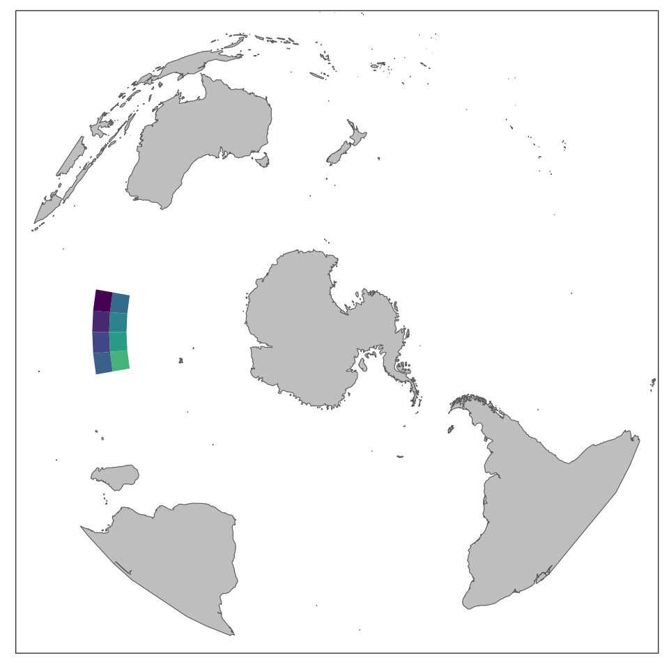

Figure - map of overall observed effort

# Map of observed effort by month

# get observed effort by cell
plt_dat <- obs_data %>%
  st_drop_geometry(.) %>%
  group_by(., id_cell, id_month) %>%
  summarise(., observer_effort = sum(observer_effort)) %>%
  ungroup(.)

# add geometry from grid
plt_dat <- plt_dat %>% left_join(., grid, by = "id_cell") %>% st_as_sf(.)

# generate plot
plt <- ggplot(plt_dat) +
  geom_sf(aes(fill = observer_effort), col = NA) +
  guides(fill = "none") +
  scale_fill_viridis_c("Observed\neffort", direction = -1, limits = c(0, NA)) +
  facet_wrap(vars(id_month), nrow = 4, ncol = 3) +
  theme_sh()

ggsave(paste0("map_observed_effort_by_month_", flag_str_label, ".png"), plot = plt, device = "png",
       path = figures_path, width = 5, height = 5, units = "in")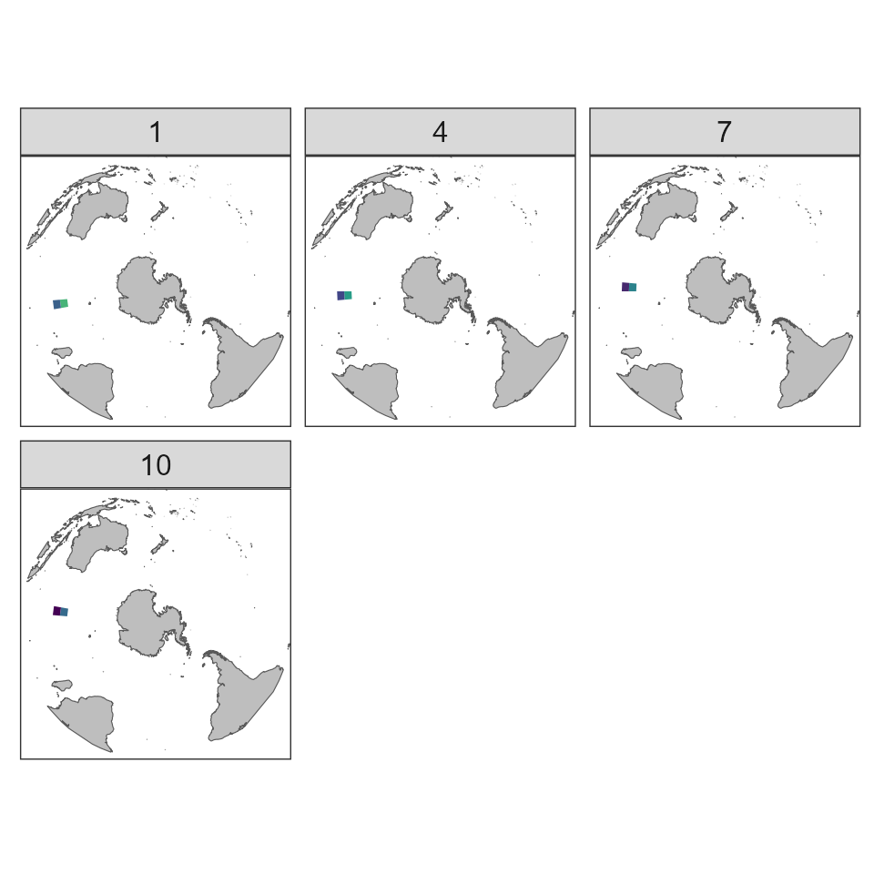

Figure - map of overall observed effort by month

# Map of observed effort by fishery group
if(nrow(lk_fishery_groups) > 1) {

  # get observed effort by cell
  plt_dat <- obs_data %>%
    st_drop_geometry(.) %>%
    group_by(., id_cell, id_fishery_group) %>%
    summarise(., observer_effort = sum(observer_effort)) %>%
    ungroup(.)

  plt_dat <- plt_dat %>% left_join(., lk_fishery_groups, by = "id_fishery_group")

  # add geometry from grid
  plt_dat <- plt_dat %>% left_join(., grid, by = "id_cell") %>% st_as_sf(.)

  # generate plot
  plt <- ggplot(plt_dat) +
    geom_sf(aes(fill = observer_effort), col = NA) +
    guides(fill = "none") +
    scale_fill_viridis_c("Observed\neffort", direction = -1) +
    facet_wrap(vars(fishery_group), nrow = nrow(lk_fishery_groups), ncol = 1) +
    theme_sh()

  ggsave(paste0("map_observed_effort_by_fgroup_", flag_str_label, ".png"), plot = plt, device = "png",
         path = figures_path, width = 5, height = 5.5 * nrow(lk_fishery_groups), units = "in")
}

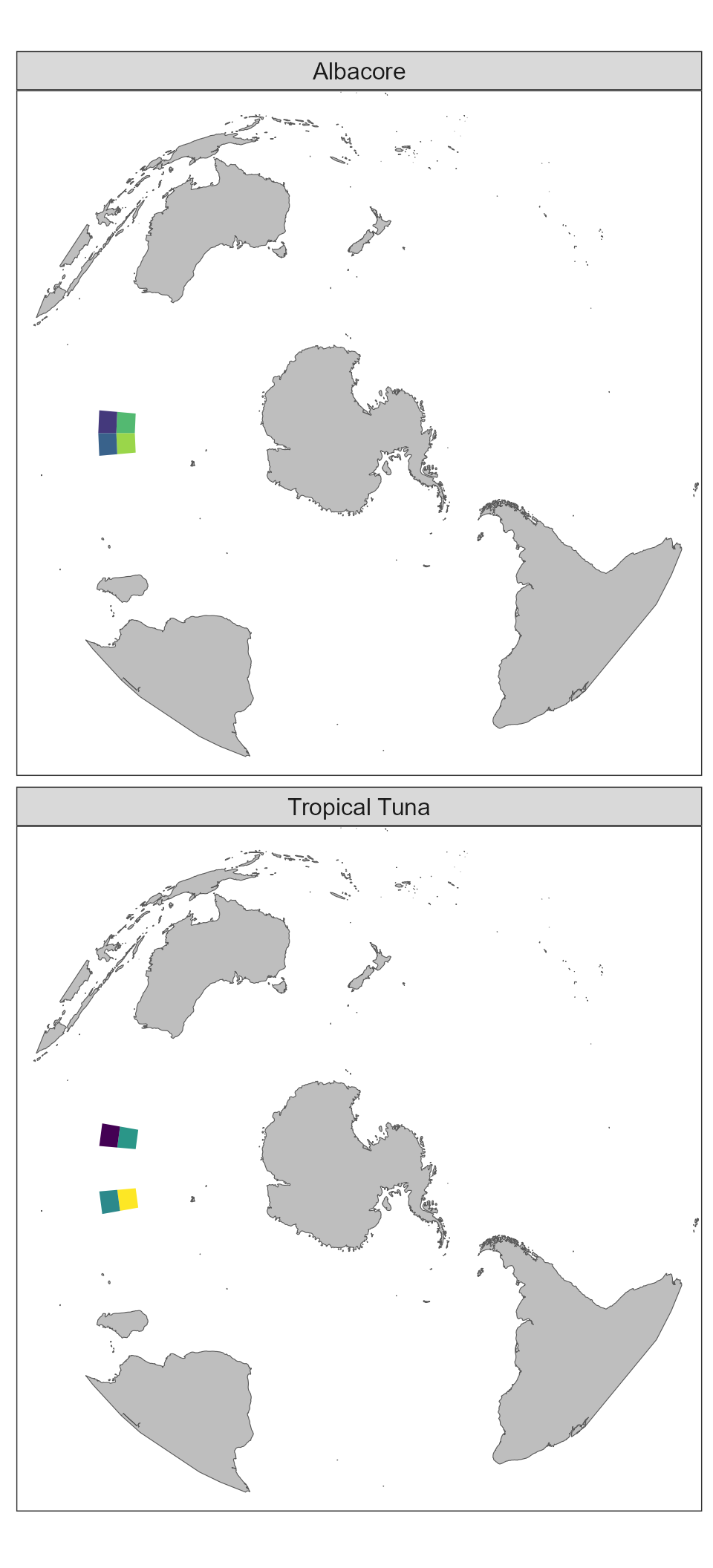
Figure - map of overall observed effort by fishery group

# Map of observed effort by time period
if(nrow(lk_time_periods) > 1) {

  # get observed effort by cell
  plt_dat <- obs_data %>%
    st_drop_geometry(.) %>%
    group_by(., id_cell, id_period) %>%
    summarise(., observer_effort = sum(observer_effort)) %>%
    ungroup(.)

  plt_dat <- plt_dat %>% left_join(., lk_time_periods, by = "id_period")

  # add geometry from grid
  plt_dat <- plt_dat %>% left_join(., grid, by = "id_cell") %>% st_as_sf(.)

  # generate plot
  plt <- ggplot(plt_dat) +
    geom_sf(aes(fill = observer_effort), col = NA) +
    guides(fill = "none") +
    scale_fill_viridis_c("Observed\neffort", direction = -1) +
    facet_wrap(vars(period), nrow = nrow(lk_time_periods), ncol = 1) +
    theme_sh()

  ggsave(paste0("map_observed_effort_by_period_", flag_str_label, ".png"), plot = plt, device = "png",
         path = figures_path, width = 5, height = 5.5 * nrow(lk_time_periods), units = "in")
}

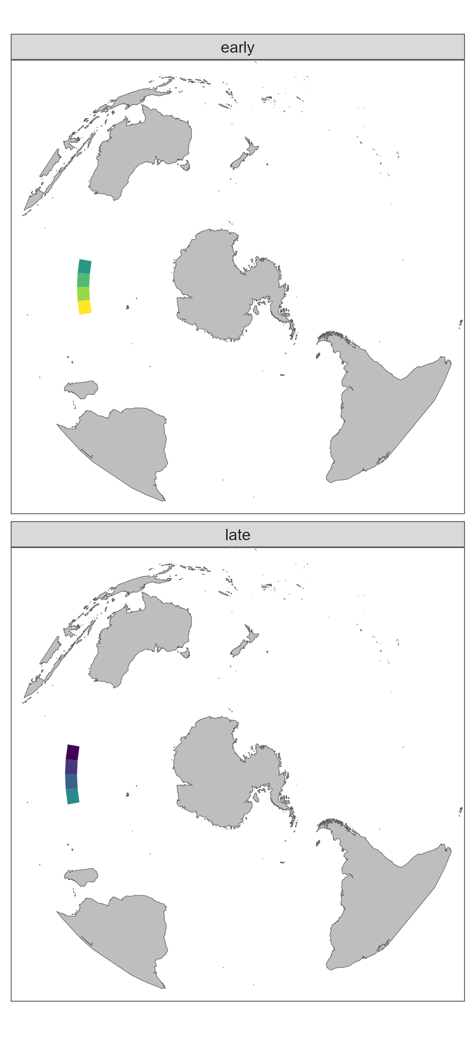
Figure - map of overall observed effort by time period

Save prepared data

Save processed observer data at a raw (i.e., un-aggregated) resolution:

save(obs_data, file = file.path(dir_data, "obs_data.rda"))
save(obs_overlap, file = file.path(dir_data, "obs_overlap.rda"))

obs_data and obs_overlap are not required as an input for the risk assessment model, but may be of interest to the User.

Save inputs to the risk assessment model

Save observed overlap:

save(overlap_o, file = file.path(dir_data, "overlap_o.rda"))

Save captures data:

save(captures_o, file = file.path(dir_data, "captures_o.rda"))

Issues preparing your data

If you encounter any issues preparing your observer dataset, please create a new Issue for the sefraInputs Github repository with a description of the problem, including any error messages, and one of the project team will assist.